<?xml version="1.0" encoding="utf-8"?><feed xmlns="http://www.w3.org/2005/Atom" ><generator uri="https://jekyllrb.com/" version="3.10.0">Jekyll</generator><link href="https://plewandow.ski/feed.xml" rel="self" type="application/atom+xml" /><link href="https://plewandow.ski/" rel="alternate" type="text/html" /><updated>2026-08-25T20:55:46+02:00</updated><id>https://plewandow.ski/feed.xml</id><title type="html">Piotr Lewandowski</title><subtitle>Piotr Lewandowski - Blog</subtitle><author><name>Piotr Lewandowski</name><email>piotr.w.lewandowski@gmail.com</email></author><entry><title type="html">Notes on ‘‘Asynchronous Entanglement Routing for the Quantum Internet’’</title><link href="https://plewandow.ski/quantum%20computing/routing/quantum%20routing/quantum-async-routing-notes/" rel="alternate" type="text/html" title="Notes on ‘‘Asynchronous Entanglement Routing for the Quantum Internet’’" /><published>2024-03-06T00:00:00+01:00</published><updated>2024-03-06T00:00:00+01:00</updated><id>https://plewandow.ski/quantum%20computing/routing/quantum%20routing/quantum-async-routing-notes</id><content type="html" xml:base="https://plewandow.ski/quantum%20computing/routing/quantum%20routing/quantum-async-routing-notes/"><![CDATA[<h1 id="overview">Overview</h1>

<p>Goal of this post is to describe <a href="https://arxiv.org/abs/2312.14300">Asynchronous Entanglement Routing for the Quantum Internet</a> with focus on the results <em>and</em> open problems. The post will be structured in a following way – in the first section I will describe (on a high level) problem that is being addressed in the main article, in the second section we will go through foundational blocks and context required to understand the paper, in third section I will describe main contribution from the paper, fourth section will contain details about simulation setup and results, fifth section will contain open problems as described in the paper.</p>

<h2 id="why-this-particular-structure">Why this particular structure?</h2>

<p>I believe this approach facilitate better understand - both for reader and for me as a writer of this notes. Having clear picture of <em>what particular problem</em> authors are trying to solve is critical to understanding the solution and somewhat appreciate it. Then, before diving into main contribution (which is a solution to a stated problem), we need to ensure that we are standing on solid foundation. Usually parts like ‘‘Section II’’ are bit boring, yet they are helpful to fully grasp solution described in ‘‘Section III’’.</p>

<h1 id="section-i-problem-definition">Section I: Problem definition</h1>

<p>Given set of ‘‘quantum devices’’ (capable of entanglement generation and swapping) connected via network capable of qubit transmission – how we can <em>efficiently</em> create entanglement between any two devices in the network?</p>

<h2 id="context">Context</h2>

<p>In the article it is Section 3. ‘‘Quantum network’’ is a network – mathematically represented by a graph – which leverages some quantum specific properties, in this case <a href="https://en.wikipedia.org/wiki/Quantum_entanglement">entanglement</a>. Graph $G(V, E)$ consists of a set of <em>vertices</em> $V$ (nodes, ‘‘quantum devices’’) and a set of <em>edges</em> $E$ (fibers, connection between nodes). Entanglement gives us possibility to create also <em>virtual edges</em> between particular vertices. Let us focus on that - what is a virtual edge? We will consider simple graph consisting of three nodes - $A, B, C$. The solid lines represents physical link between two devices.</p>

<pre><code class="language-mermaid">graph LR;
    A---B;
    B---C;
</code></pre>

<p>Now, each node represents quantum device. Each device can communicate <em>qubits</em> to its neighbour (so another node that is directly connected). Such pair of nodes can create entanglement between their states. In our graph we (in theory) entangle states of $A, B$ and $B, C$. We will represent entanglement between nodes with dotted line.</p>
<pre><code class="language-mermaid">graph LR;
    A---B;
    B---C;
    A-.-B;
    B-.-C;

</code></pre>

<p>By using technique called <em>entanglement swapping</em> we can “sacrifice” entanglements between $A, B$ and $B, C$ to create entanglement between $A, C$!</p>

<pre><code class="language-mermaid">graph LR;
    A---B;
    B---C;
    A-.-C;
</code></pre>

<p>What’s the benefit? Now pair $A, C$ is entangled and they can leverage ‘‘quantum effects’’ - for example in quantum key distribution. Of course as networks grow larger, keeping in mind intermittent and delicate nature of entanglement between nodes, the question of how to create entanglement between any two particular nodes in a network gets harder and harder. Hence, we get our original problem statement.</p>

<h1 id="section-ii-prerequisites-and-problem-statement-refinement">Section II: Prerequisites and problem statement refinement</h1>

<p>Before we can fully jump into contribution of the paper we need to understand what <em>building blocks</em> are leveraged in proposed approach. First we will describe processes or ‘‘functions’’, then we will describe components that leverage these.</p>

<h2 id="entanglement-generation-between-adjacent-nodes">Entanglement generation between adjacent nodes</h2>

<p>Most basic capability is to entangle qubits between two adjacent nodes in a network. Simplest way would be to generate <a href="https://en.wikipedia.org/wiki/Bell_state#Creating_Bell_states_via_quantum_circuits">EPR pair</a> between in node $A$ and then send one of the entangled qubits to connected (via physical link) node $B$.</p>

<h2 id="entanglement-swapping">Entanglement swapping</h2>

<p>With the information above we can generate entanglement between physically connected nodes, but what about situation where we have intermediary node?</p>

<pre><code class="language-mermaid">graph LR;
  subgraph PRE[from this]
     A-.-B
     A---B
     B-.-C
     B---C
   end
   subgraph POST[to this]
     D[A]---E[B]
     E---F[C]
     D-.-F
   end

PRE --&gt; POST
</code></pre>

<p>There is existing technique called <a href="https://en.wikipedia.org/wiki/Quantum_teleportation#Entanglement_swapping">entanglement swapping</a>, which allows us to do exactly that. In linked example there is a
algorithmic description of the process, whereas in the paper you can find circuit-level realisation.</p>

<h2 id="fidelity">Fidelity</h2>

<p>Fidelity between two quantum states can be intuited as “similarity” between those two states. Higher fidelity between two states means that two states are more similar to each other. In case of pure states fidelity can be thought as angle between two vector states.</p>

<h2 id="entanglement-purification">Entanglement purification</h2>

<p>This is a procedure that takes a number of partially entangled states and produces a smaller number (not rarely - just one) state with higher measure of entanglement.</p>

<h2 id="global-and-local-node-level-knowledge-of-direct-links">Global and local (node-level) knowledge of direct links</h2>

<p>First - what is a direct link? Given two nodes in the network, “direct link” is an edge realised by entanglement between those two nodes.
The “global knowledge” is information about states of all direct links between all nodes in the network. It completely describes entanglement between all nodes. In a perfect (yet somewhat imaginary) world every node would have access to that global knowledge, but in a distributed scenario - the state information in any node might be outdated hence it has a “local knowledge”. If you are coming from CS perspective - this simply means <a href="https://en.wikipedia.org/wiki/Eventual_consistency">eventual consistency</a></p>

<h2 id="link-capacity">Link capacity</h2>

<p>This is a number representing how many entangled qubit pairs can be generated between two nodes. If we would have ‘‘prefect’’ technology it would simply be equal to number of pairs between two nodes, but physical realisation within current state of the art implies that  – if we want to achieve specific fidelity with EPR pair – we might need multiple entangled pairs and leverage purification techniques.</p>

<h2 id="synchronous-and-asynchronous">Synchronous and asynchronous</h2>

<p>Title of the article contains “asynchronous”, hence it would be good to explain what does it mean. From a programmer perspective (or <em>thread</em> perspective) synchronous means that you wait for task to finish before working on next task. When you execute some task asynchronously - you can delegate the work to another ‘‘thread’’ (or other entity of similar type) and work on something else between you get the result back.</p>

<p>Overall, this is a very deep ocean, especially in world of algorithm analysis – so let us try to narrow down what it does mean in context of the paper. It simply means that nodes in the network can perform operations (for example - creating entanglement) simultaneously, without any “global” coordination.</p>

<p>On the page 3, authors mention that existing (synchronous) approaches are generally divided in two phases – external and internal. During the “external” phase, adjacent nodes establish entanglement between each other. During the “internal” phase – nodes are only aware of entanglement status of their neighbours – (quoting from article) “each repeater node swaps entanglement blindly to reach an end-to-end entanglement” between source and target nodes. If the source-target connection is not achieved, process is repeated. The “synchronous” aspect comes from the fact that internal phase needs all entanglement links built in external phase. Moreover, <em>all entanglements</em> are consumed in each time slot. Time slot consists of external + internal phase.</p>

<h2 id="entanglement-rate">Entanglement rate</h2>

<p>This value represents how much entanglement can be generated in a unit of time. Paraphrasing from paper: <em>It is the performance metric indicating the number of end-to-end entanglements (Bell states) that can be generated in a unit time $T$</em>.</p>

<h2 id="refined-problem-statement">Refined problem statement</h2>

<p>This section will contain more mathematically precise statement of the problem. It is heavily based on Section 3 of the paper.</p>

<p>Let graph $G(V, E)$ represent topology of a quantum network. Each node $v \in V$ represents a quantum repeater (capable of entanglement generation and swapping), while each edge $e \in E$ represents physical (e.g. fiber optic) node that connects two repeaters. Let $G’(V’, E’)$ be a graph, where $V’ \subseteq V$. $G’$ represents quantum repeaters that are connected with each other via direct entanglement. Hence $e’ \in E’$ represents entanglement connection (in the paper this is called ‘‘direct-link entanglement’’).</p>

<p>Each edge $e \in E$ has associated value $C(e)$ which represents <em>capacity</em> of the link. Capacity is defined as maximum number of entangled pairs that can be generated between nodes connected by $e$. Moreover, each vertex $v \in V’$ also has capacity - $C(v)$, which is defined simply as number of qubits in that particular vertex (remember - vertex is simply a quantum repeater). $C(v)$ is defined as at least equal to sum of capacities of edges that connect $v$ with its neighbours $N(v)$. $C(v) \geq \sum_{e \in N(v)}C(e)$. This will allow us to simplify analysis, because there is no “competition” for qubits between links.</p>

<p>As mentioned before due to limitations of our technology to achieve desired fidelity $f$ (with EPR pair), we need $E(f)$ entanglement pairs to obtain it (via purification). We also define $T_{co}$, which is an <em>average coherence time</em>. It can be understood as how long we can actually maintain entanglement. After that time (on average) we will loose entanglement between two nodes.</p>

<p>In the paper - to simplify the analysis - each link capacity $C(e)$ and $E(f)$ are equal to $1$.</p>

<p>For each entanglement generation that happens between nodes connected via edge $e$ there is probability $p(e)$ that generation will succeed. At each node $v$ there is probability of entanglement swapping succeeding denoted as $q(v)$. To simplify things authors of the paper denote equal $p(e)$ for all edges $e$ – denoted simply as $p$. Analogously, $q$ represents success probability for entanglement swapping for all $v$.</p>

<p>Entanglement rate $\zeta$ represents number of Bell states that can be generated in unit time $T \leq T_{co}$. This last inequality makes sense, because it allow us to narrow down time window to only consider generation of entanglements that all can “live” at the same time.</p>

<p>Moreover, additional (but important) constraint that authors put on themselves is that nodes only posses local knowledge about adjacent entanglement links.</p>

<p>So the refined problem statement would be - given all of the above and assuming asynchronicity - how to design an algorithm that maximizes entanglement rate $\zeta$.</p>

<h1 id="section-iii-main-contributions">Section III: Main contributions</h1>

<p>Before we dive into particular contributions, let us go through various ideas, tools and constructs used by authors to better understand main results</p>

<h2 id="connected-oriented-circuit-switching-vs-connection-less-packet-switching">Connected-oriented circuit switching vs connection-less packet switching</h2>

<p>I think one of the sentences gives good insight into inspiration for the approach taken by the authors (Section 3, page 8):</p>

<blockquote>
  <p>characteristic of entanglement resembles connection-oriented circuit switching rather than the connection-less packet switching used in classical networking.</p>
</blockquote>

<p>Given that this is important let’s understand what is <em>connection-oriented circuit switching</em> and <em>connection-less packet switching</em>.</p>

<p>First the latter one.</p>

<p>In connection-less packet switching data is divided into <em>packets</em> and each such <em>packet</em> is treated independent unit. There is no pre-established path for data transmission for every packet. Packets may take different routes to reach the destination, and they might arrive out of order. The network nodes make routing decisions based on the current network conditions.</p>

<p>In connection-oriented circuit switching a dedicated communication path (known as circuit) is established between two parties before any data transfer occurs. The path remains reserved for the duration of the connection.</p>

<p>The entanglement cannot be split into parts, we need to reserve particular path to entangle nodes connected by that path. That’s why the connected oriented approach seems like a more natural fit.</p>
<h2 id="dodag">DODAG</h2>

<p>DODAG is an acronym that stands for <em>destination oriented directed acyclic graph</em>. The DAG part is usually well-known, especially in computer science world. The core property of DAG is having directed edges which form a path <em>without</em> cycles. So going on any path on that graph will not bring you to place you’ve been before.</p>

<p>DODAG is a specific type of DAG that is leveraged in lossy networks (think of dynamic IoT scenario). The additional property to designate one of the vertices as a <em>root node</em> that will have no outgoing edges. All other nodes in the graph can be reached from the root by following the directed edges.</p>

<h2 id="spanning-tree">Spanning tree</h2>

<p>Spanning tree will also be leveraged within the paper. Given graph $G(V, E)$ its spanning tree is another graph that contains the same set of vertices $V$, <em>but</em> it contains minimum possible number of edges to retain same connections as original graph have (connection here means being able to go from vertex $a$ to vertex $b$)</p>

<h2 id="distributed-graph">Distributed graph</h2>

<p>Distributed graph is a type of graph where each vertex/node is a <em>computing unit</em> – in our case it is a quantum repeater.</p>

<h2 id="instant-topology">Instant topology</h2>

<p>Instant topology refers to a topology of a graph that is built from quantum repeater (nodes) that are connected via entanglement (edges)</p>

<h2 id="getting-to-the-point">Getting to the point</h2>

<p>With that long preface and all concepts, we can finally get to describing the key results of the paper. Whew!</p>

<h3 id="key-idea">Key idea</h3>

<p>This is based heavily on section 4 of the article.</p>

<p>I think that good mental model for the <em>asynchronous routing scheme</em> is a service (from software perspective). It is constantly “on” and reacts to particular queries (simplest example is some form of simple http server).</p>

<p>This “routing service” is built from two main components: distributed graph and path determinator.</p>

<p>First component – the “distributed graph” – is responsible for building and maintaining instant topology as a distributed graph. Second component is more of a server which respond to actual requests. If you are software engineering savvy, this routing scheme have traits of a reactive system.</p>

<p>Given my personal software engineering context, I’ll try to represent the scheme in a pseudocode.An instance of class below would run on every node/vertex/quantum repeater in the network.</p>

<div class="language-python highlighter-rouge"><div class="highlight"><pre class="highlight"><code><table class="rouge-table"><tbody><tr><td class="rouge-gutter gl"><pre class="lineno">1
2
3
4
5
6
7
8
9
10
11
12
13
14
15
16
17
18
19
20
21
22
23
24
</pre></td><td class="rouge-code"><pre><span class="k">class</span> <span class="nc">AsynchronousRouterNode</span><span class="p">:</span>
    <span class="n">distributed_graph_component</span> <span class="c1"># responsible for building and maintaining instant topology 
</span>    <span class="n">current_node</span> <span class="o">=</span> <span class="bp">self</span>

    <span class="c1"># On instance startup
</span>    <span class="k">def</span> <span class="nf">startup</span><span class="p">():</span>
        <span class="n">distributed_graph_component</span><span class="p">.</span><span class="n">join</span><span class="p">(</span><span class="n">current_node</span><span class="p">)</span>

    <span class="c1"># This function would be called as a classical operation with "classical bits"
</span>    <span class="k">def</span> <span class="nf">navigate</span><span class="p">(</span><span class="n">previous_node</span><span class="p">,</span> <span class="n">destination_node</span><span class="p">):</span>
        <span class="n">maybe_next_node</span> <span class="o">=</span> <span class="n">distributed_graph_component</span><span class="p">.</span><span class="n">next_hop_determination</span><span class="p">(</span><span class="n">current_node</span><span class="p">,</span> <span class="n">destination_node</span><span class="p">)</span>
        <span class="k">if</span> <span class="n">maybe_next_node</span> <span class="ow">is</span> <span class="bp">None</span><span class="p">:</span>
            <span class="c1"># a naive retry - try to join this node to distributed graph and retry the request
</span>            <span class="n">distributed_graph_component</span><span class="p">.</span><span class="n">join</span><span class="p">(</span><span class="n">current_node</span><span class="p">)</span>
            <span class="n">navigate</span><span class="p">(</span><span class="n">previous_node</span><span class="p">,</span> <span class="n">destination_node</span><span class="p">)</span>
        <span class="k">else</span><span class="p">:</span>
            <span class="n">next_node</span> <span class="o">=</span> <span class="n">maybe_next_node</span>
            <span class="n">es_success</span> <span class="o">=</span> <span class="n">entanglement_swap</span><span class="p">(</span><span class="n">previous_node</span><span class="p">,</span> <span class="n">next_node</span><span class="p">)</span>
            <span class="k">if</span> <span class="ow">not</span> <span class="n">es_success</span><span class="p">:</span> <span class="c1"># if entanglement swapping failed
</span>                <span class="c1"># once again - a naive retry.
</span>                <span class="n">distributed_graph_component</span><span class="p">.</span><span class="n">join</span><span class="p">(</span><span class="n">current_node</span><span class="p">)</span>
                <span class="n">navigate</span><span class="p">(</span><span class="n">previous_node</span><span class="p">,</span> <span class="n">destination_node</span><span class="p">)</span>
            <span class="k">else</span><span class="p">:</span>
                <span class="n">emit_connection_request_to</span><span class="p">(</span><span class="n">next_node</span><span class="p">,</span> <span class="n">destination_node</span><span class="p">,</span> <span class="n">current_node</span><span class="p">)</span>
</pre></td></tr></tbody></table></code></pre></div></div>

<p>This relatively short pseudocode gives good overview and shows that even if we get complicated behavior (asynchronous entanglement swapping) behaviour of an individual node is simple:</p>
<ol>
  <li>On startup connect to the <code class="language-plaintext highlighter-rouge">distributed_graph_component</code></li>
  <li>On request – try to swap entanglement between previous node and next node. Here the important part is that <code class="language-plaintext highlighter-rouge">distributed_graph_component</code> maintains information about instant topology (where edges represents entanglement between nodes). If something fails - try to rejoin the graph and retry the request.</li>
</ol>

<p>We can see an unsafe infinite loop here (infinite retry), but this is of course just a pseudocode, so I can live with that.</p>

<p>The important questions that arises - how we can realise the <code class="language-plaintext highlighter-rouge">distributed_graph_component</code>. From perspective of individual node this is completely opaque, but of course - we are interested in performance on an <em>actual</em> solution. Authors propose two “protocols” that implements the component – DODAG and Spanning Tree. I believe it is worthwhile to understand both approaches (at least on a high level). On the other hand there is possibility to implement other protocols as we develop the science behind it. For detailed explanation please refer to the paper - esp. section 4.</p>

<p>To give even more intuition on “how this works” let me quote from the conclusion section:
“We treat all network nodes as vertices in a graph that try to connect their neighbours using direct-link entanglements. No central control and no global knowledge of the direct-link entanglements are needed in our method. Whenever a pair of nodes wants to create an end-to-end entanglement, they go through the distributed graph that is continuously updated to find each other”</p>

<h1 id="section-iv-simulation-setup-and-results">Section IV: Simulation setup and results</h1>

<p>Now to the results. Authors provided interesting model, especially the fact that it moves towards asynchronicity – which seems like a more natural fit for a network. The question remains if it is better than the synchronous approach.</p>

<h2 id="experiment-setup">Experiment setup</h2>

<p>Authors utilise entanglement rate (as defined above) $\zeta$ as a performance metric. They run the experiment on a 2D grid topology. Each node is connected to 4 other nodes (neighbours), with exception of edge nodes (those are connected to 3 neighbours) and ‘‘corners’’ (those are connected to 2 neighbors). Each node is only aware of the neighbours’ statuses of entanglement (direct links in an instant topology) and has <em>no</em> awareness about anything “larger” than that.</p>

<p>Authors use <a href="https://networkx.org/">NetworkX</a> python library to conduct the simulation. Simulation happens (as mentioned above) in a 2D grid network. It is not clearly stated in the paper what is the size of the grid, but from the description of the Figure 10, we might think that it is around $26 \times 26$.</p>

<h2 id="synchronous-protocol">Synchronous protocol</h2>

<p>Authors compare results to “synchronous” protocol. Authors do not describe precisely what protocol they are comparing against, so I assume that they leverage what they described in section 5.1. For us the main interest would be entanglement rate in synchronous protocol:</p>

\[\zeta_{syn}(s, t) = p^{l_{s,t}}q^{l_{s,t}-1}n_{s,t}\]

<p>Let us unpack:</p>
<ul>
  <li>$s$ means source node</li>
  <li>$t$ is target node</li>
  <li>$p$ is probability of success of entanglement between adjacent nodes</li>
  <li>$q$ is probability of success of entanglement swap</li>
  <li>$l_{s,t}$ is the mean length of all possible paths between nodes $s$ and $t$</li>
  <li>$n_{s,t}$ average number of disjoint paths between $s$ and $t$ as $n_{s,t}$</li>
</ul>

<h2 id="on-t_co">On $T_{co}$</h2>

<p>To fully grasp simulation results, how coherence time – $T_{co}$ – is leveraged. $T_{co}$ represents coherence time or “how long entanglement is alive and usable”. Entanglement <em>rate</em> means that we are talking about how much entanglement we can generate per unit time $T$. For simulations (and analysis) to be meaningful we must assume that $T \leq T_{co}$ – otherwise we would not have available entanglement after single time unit. Authors decided to represent $T_{co}$ as $n$ unit times, so $T_{co} = 3$ represents coherence time of 3 unit times. Unit time is equivalent to ‘‘one time slot in synchronous operation’’, but it is not clearly defined what it means. Entanglement rate for synchronous protocol is independent of $T_{co}$.</p>

<h2 id="results">Results</h2>

<blockquote>
  <p>Graphs are taken from <a href="https://arxiv.org/abs/2312.14300">Asynchronous Entanglement Routing for the Quantum Internet</a></p>
</blockquote>

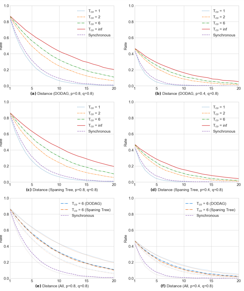
<h3 id="rate-vs-distance-single-path">Rate vs Distance (single-path)</h3>

<p><img src="/assets/img/async_quantum_routing/simulation_results.jpg" alt="Simulation Results" title="simulation_results" /></p>

<p>Single-path means that we search only for one path between source and destination nodes.</p>

<p>First thing to notice is that for $T_{co} = 1$ synchronous approach beats asynchronous one. It makes sense, as there is an “additional baggage” for async communication – which does not exist in synchronous approach. But, with $T_{co} = 2$ asynchronous protocols are beating synchronous approach.</p>

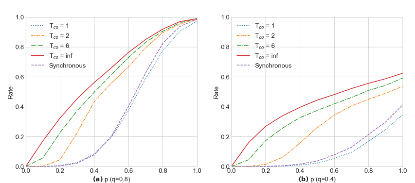
<h3 id="rate-vs-entanglement-generation-success">Rate vs Entanglement Generation success</h3>

<p><img src="/assets/img/async_quantum_routing/p_simulation_results.png" alt="Q simulation results" title="p_simulation_results" /></p>

<p>Here we can see similar results – async approaches are better when coherence time increases, interesting question is that if we $p$ and $q$ approach $1$ - would we observe any difference? Graph on the left shows that with high values of $p$ and $q = 0.8$ we see almost no difference.</p>

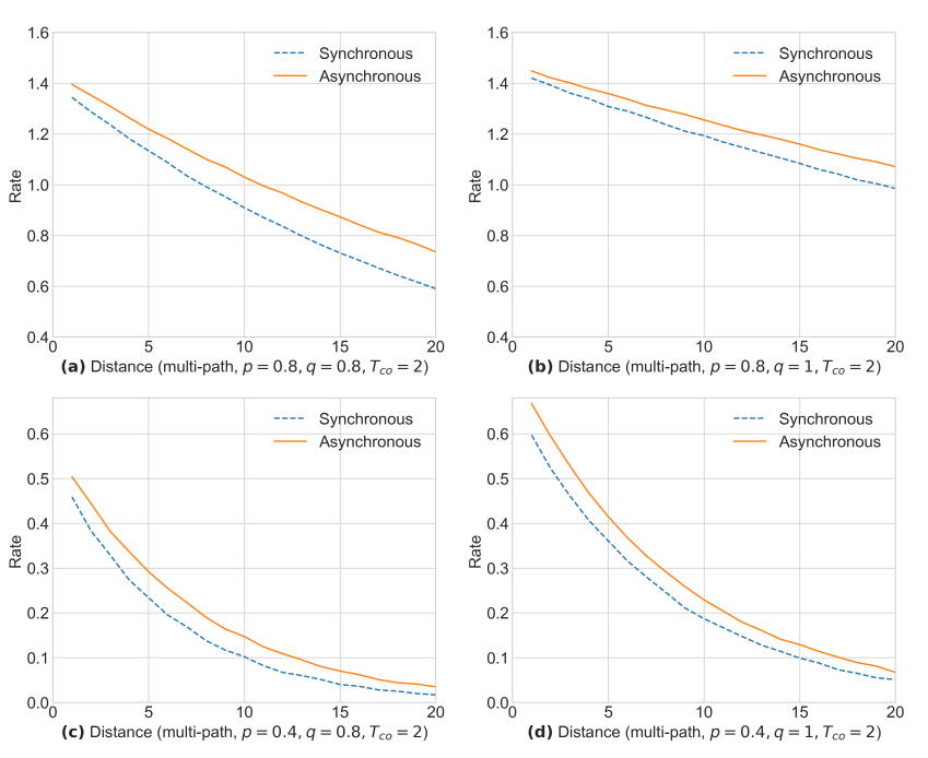
<h3 id="rate-vs-distance-multi-path">Rate vs Distance (multi-path)</h3>

<p><img src="/assets/img/async_quantum_routing/multi_path_results.jpg" alt="multi path simulation results" title="multi_path_results" /></p>

<p>Multi-path means that we search for disjoint paths between source and target nodes. Once again the async approaches beat synchronous approach (but not that much).</p>

<h1 id="section-v-open-problems-future-work-and-potential-directions">Section V: Open problems, future work and potential directions</h1>

<h2 id="network-of-networks">Network of networks</h2>

<p>Authors claim that DODAG roots can serve as gateways to connect multiple networks (constructing network of networks). Leveraging DODAG for async routing (as presented in this article) of network of networks is a direction for future exploration.</p>

<h2 id="root-position">Root position</h2>

<p>Authors took center of the network as DODAG’s root, but taking different nodes as roots and impact of that decision on entanglement rate warrants further investigation.</p>

<h2 id="networking-properties">Networking properties</h2>

<p>Aspects like using (quoting/paraphrasing) “untrusted repeaters, minimal trust between network, malicious nodes, order of entanglement swapping along a path”</p>

<h2 id="network-shapes">Network shapes</h2>

<p>Performance of routing schemes in networks with shape other than grid.</p>

<h3 id="personal-propositions">Personal propositions</h3>

<ul>
  <li>Are there different structures other than DODAG?</li>
  <li>What results for $T_{co} \in (1, 2)$?</li>
  <li>More granular comparisons with different synchronous algorithms</li>
  <li>(far-fetched) can we learn something from blockchain related research?</li>
</ul>]]></content><author><name>Piotr Lewandowski</name><email>piotr.w.lewandowski@gmail.com</email></author><category term="quantum computing" /><category term="routing" /><category term="quantum routing" /><category term="quantum" /><category term="routing" /><category term="theory" /><category term="notes" /><summary type="html"><![CDATA[Let's try to understand article that presents more ''modern'' approach to creating entanglement between any two nodes in a quantum network]]></summary></entry><entry><title type="html">Notes on (Part 1 of) Lemma 4.1 from ‘‘Computational Quantum Entanglement paper’’</title><link href="https://plewandow.ski/quantum%20computing/computational%20quantum%20entanglement/seperation-proof-cet/" rel="alternate" type="text/html" title="Notes on (Part 1 of) Lemma 4.1 from ‘‘Computational Quantum Entanglement paper’’" /><published>2024-01-08T00:00:00+01:00</published><updated>2024-01-08T00:00:00+01:00</updated><id>https://plewandow.ski/quantum%20computing/computational%20quantum%20entanglement/seperation-proof-cet</id><content type="html" xml:base="https://plewandow.ski/quantum%20computing/computational%20quantum%20entanglement/seperation-proof-cet/"><![CDATA[<p><strong>Big thank you to professors Karol Horodecki and Thomas Vidick for helping me understand all the parts of the proof.</strong></p>

<p>Below are my notes on the proof of Lemma 4.1 from the paper <a href="https://arxiv.org/abs/2310.02783">Computational Quantum Entanglement</a>. My approach is to take the proof apart and try to understand each step. I will try to explain the concepts in a way that is understandable for me. Each part will be taken as a $\textit{claim}$ and I will try to convince myself why it is true.</p>

<p>Here I will focus only on proving bounds on part regarding (computational) entanglement distillation.</p>

<h2 id="what-are-we-trying-to-prove">What are we trying to prove?</h2>

<blockquote>
  <p>For any small enough $\varepsilon &gt; 0$ and non-decreasing $n(\lambda)$ such that $n(\lambda) \rightarrow \infty$ as $\lambda \rightarrow \infty$, 
there exists a family $\{\rho_{\lambda}^{AB}\}$ of bipartite pure states on $2n(\lambda)$ qubits such that for all $\lambda$, 
$E_{D}^{0}(\rho_{\lambda}^{AB}) = E(\rho_{\lambda}^{A}) = n(\lambda)$, but for any valid lower bound $m$ on 
$\hat{E_{D}}^{0}(\rho_{\lambda})$, we have that $m \leq_{\infty} 0$.</p>
</blockquote>

<h3 id="what-does-it-mean">What does it mean?</h3>

<p>There exist a family of states $\{\rho_{\lambda}^{AB}\}$ that has high (namely $n(\lambda)$) distillable entanglement , but small (namely 0) <em>computational</em> distillable entanglement.</p>

<h2 id="intuitive-proof-overview">Intuitive proof overview</h2>

<p>To distill entanglement we need to create at least single EPR pair. 
The idea is to create a family of pure states (of which uniform mixture is the totally mixed state) that is way more numerous than number of efficient LOCC maps from those states to one EPR pair.
If the family has so many states that <em>almost all</em> (at least half of them) of them would be distilled by one (family parametrized by $\lambda$ of) LOCC map.
Assume that this <em>efficient</em> (critical part of assumption) LOCC map actually exist. Then, this particular LOCC map by being linear should also distill with non-zero fidelity from uniform mixture of the family - from this we have non-zero distillable entanglement. But we know that totally mixed state has
entanglement entropy (via entanglement of formation) equal to 0. Entanglement entropy is an upper bound for distillable entanglement, hence we arrive at contradiction.</p>

<h3 id="what-is-the-post">What is the post:</h3>

<ul>
  <li>Claims 1, 2 describe why we can even think about constructing such family of states</li>
  <li>Claim 3 shows that this family of state might be very populated.</li>
  <li>Claims 4, 4.1, 4.2, 4.3, 4.4 show properties of such family of states.</li>
  <li>Claims 5.1, 5.2 are the “actual” proofs.</li>
</ul>

<h2 id="claim-1-for-n-qubits-unitaries-u-and-v-and-lvert-phin-rangle-the-tensor-product-of-n-epr-pairs-the-states-i-otimes-ulvert-phin-rangle-and-i-otimes-vlvert-phin-rangle-are-both-maximally-entangled">Claim 1: For $n$-qubits unitaries $U$ and $V$, and $\lvert \phi^n \rangle$ the tensor product of $n$ EPR pairs, the states $(I \otimes U)\lvert \phi^n \rangle$ and $(I \otimes V)\lvert \phi^n \rangle$ are both maximally entangled.</h2>

<p>If you are into quantum computing already, this is true because $\lvert \phi^n \rangle$ is maximally entangled (by definition of EPR pair) and
we cannot “change” entanglement by using local operations – and those what $(I \otimes V)$ are. We apply each <em>same</em> unitary to each EPR pair.</p>

<p>I personally prefer more mathematical oriented proofs.</p>

<p>To show that state $(I \otimes U)\lvert \phi^n \rangle$ is maximally entangled, we need to show that reduced density operator for subysystem will not change.</p>

<p>First, let us consider an EPR pair - $\frac{1}{\sqrt{2}}(\lvert 00 \rangle + \lvert 11 \rangle)$. What is important to recall that this
is just a shorthand for writing $\frac{1}{\sqrt{2}}(\lvert 0\rangle_{A} \otimes \lvert 0 \rangle_{B} + \lvert 1 \rangle_{A} \otimes \lvert 1 \rangle_{B})$.
Next, $\lvert \phi^n \rangle$ is <em>actually</em> $\bigotimes_{1}^{n} \lvert \phi \rangle$. Last property that we need to leverage here is called mixed-product property and it applies to tensor (kronecker product): $(A \otimes B)(C \otimes D) = AC \otimes BD$ (if dimensions “agree”).</p>

<p>Before we go further let’s recall dimensions of used entities. $\lvert \phi \rangle$ has dimensions of $4 = 2^2 \times 1$, so  $\lvert \phi^n \rangle$ will have dimension of  $2^{2n} \times 1$. $U$ (and $V$) is an $n$-qubit unitary, so it will be $2^n \times 2^n$. So for statement $(I \otimes U)\lvert \phi^n \rangle$ to make sense $I$ needs also be a $2^n \times 2^n$ matrix.</p>

<p>Let us combine all of that and end up with (over)simplified statement</p>

\[(I \otimes U)\lvert \phi^n \rangle = (I \otimes U) \frac{1}{\sqrt{2}}^n(\sum(\lvert \alpha \rangle_A \otimes \lvert \beta \rangle_B))\]

<p>$\sum(\lvert \alpha \rangle_A \otimes \lvert \beta \rangle_B)$ – this represents a sum of all combinations that we will get from tensor-multiplying.
What is important that both (or maybe <em>each</em>) $\lvert \alpha \rangle_A$ and $\lvert \beta \rangle_B$ describe $n$-qubit system. This is why - by mixed product property we can write:</p>

\[(I \otimes U) \frac{1}{\sqrt{2}}^n(\sum(\lvert \alpha \rangle_A \otimes \lvert \beta \rangle_B)) = \frac{1}{\sqrt{2}}^n(\sum(I \lvert \alpha \rangle_A \otimes U \lvert \beta \rangle_B)) = \frac{1}{\sqrt{2}}^n(\sum(\lvert \alpha \rangle_A \otimes U \lvert \beta \rangle_B))\]

<p>That of course shows that subystem A is not affected by (I \otimes U), hence maximum entangled is retained. Of coruse exactly same reasoning can be used
for $V$.</p>

<h2 id="claim-2-states-i-otimes-ulvert-phin-rangle-and-i-otimes-vlvert-phin-rangle-have-fidelity-1--frac12frac12nlvert-u---v-rvert2_f">Claim 2: States $(I \otimes U)\lvert \phi^n \rangle$ and $(I \otimes V)\lvert \phi^n \rangle$ have fidelity $1- \frac{1}{2}\frac{1}{2^n}\lVert U - V \rVert^2_F$</h2>

<p>To be more precise, we need to show that:</p>

\[\text{Re}( \langle \phi^n \rvert (I \otimes U^H)(I \otimes V)\rvert \phi^n \rangle) = 1 - \frac{1}{2}\frac{1}{2^n}\lVert U - V \rVert^2_F\]

<p>First, let us note that both $(I \otimes U)\lvert \phi^n \rangle$ and $(I \otimes V)\lvert \phi^n \rangle$ are <em>pure</em> states – we already described them as a single ket vector in proof of previous claim (it was a sum, but that is still a single ket vector).</p>

<p>Trying to directly attack the issue via the definition of fidelity brought me nowhere, but you might now that fidelity and <a href="https://en.wikipedia.org/wiki/Trace_distance">trace distance</a> as related. Fortunately, we have the following relationship (<a href="https://en.wikipedia.org/wiki/Trace_distance#Fidelity">source</a>):</p>

\[T(\rho, \sigma) = \sqrt{1 - F(\rho, \sigma)^2} \\\]

<p>Okay, so that means that we want to show that:</p>

\[T(\rho, \sigma) = \frac{1}{2}\frac{1}{2^n}\lVert U - V \rVert^2_F\]

<p>Where $\rho$, $\sigma$ are density matrices of pure states.
Intuitively, it does make sense. We take <em>same</em> pure state, apply two different unitaries to the <em>same</em> state, hence it should be a function of distance <em>between those two unitaries</em>. Now let us define <em>trace distance</em> $T$</p>

\[T(\rho, \sigma) = \frac{1}{2}\text{Tr}(\sqrt{(\rho-\sigma)^H(\rho-\sigma)})\]

<p>Now of course – how we can prove that equality? I spent half a day with my limited mathematical skills and fell short, but fortunately I found <a href="https://arxiv.org/pdf/1903.11738.pdf">this paper</a>, from which equation 5 fell from the sky on my laps. For those sweet, sweet pure states we have:</p>

\[T(\rho, \sigma)^2 = \frac{1}{2}\lVert\rho-\sigma\rVert^2_F\]

<p>And that is something we can work with. First, let us simplify lefthand side:</p>

\[\lVert\rho-\sigma\rVert^2_F  = \text{Tr}((\rho - \sigma)^H(\rho-\sigma)) \\
= \text{Tr}(\rho^H\rho - \rho^H\sigma - \sigma^H\rho + \sigma^H\sigma) \\
= \text{Tr}(\rho - \rho^H\sigma - \sigma^H\rho + \sigma) \\
= \text{Tr}(\rho) +  \text{Tr}(\sigma) - \text{Tr}(\rho^H\sigma + \sigma^H\rho) \\
= 2 - \text{Tr}(\rho^H\sigma + \sigma^H\rho) \\
= 2 - \text{Tr}(\rho\sigma + \sigma\rho) \\
= 2 - \text{Tr}(\rho\sigma) + \text{Tr}(\sigma\rho) \\
= 2 - 2\text{Tr}(\rho\sigma) \\
= 2(1 - \text{Tr}(\rho\sigma))\]

<p>Now let’s move to $\text{Tr}(\rho\sigma)$.</p>

\[\text{Tr}(\rho\sigma) = \text{Tr}((I \otimes U)\lvert \phi^n \rangle \langle \phi^n \rvert (I \otimes U^H)(I \otimes V)\lvert \phi^n \rangle \langle \phi^n \rvert (I \otimes V^H)) \\
= \text{Tr}(\langle \phi^n \rvert(I \otimes V^H U)\lvert \phi^n \rangle \langle \phi^n \rvert (I \otimes U^HV)\lvert \phi^n \rangle)\]

<p>Now that is interesting, because both $\langle \phi^n \rvert(I \otimes V^H U)\lvert \phi^n \rangle$ and $\langle \phi^n \rvert (I \otimes U^HV)\lvert \phi^n \rangle$ are scalars, so we can drop the trace! But what is even <em>more</em> interesting is how we can leverage Exercise 9.16 from Nielsen and Chuang (be sure to check errata), Let $\lvert i \rangle, \lvert j \rangle$ be orthonormal basis set, now define $\lvert m \rangle = \sum_{i}\lvert i \rangle, \lvert j \rangle$, we get:</p>

\[\text{Tr}(A^HB) = \langle m \rvert (A \otimes B) \lvert m \rangle\]

<p>Now, let us recall that we can write $\lvert \phi^n \rangle = \frac{1}{\sqrt{2}}^n \lvert \tilde{\phi} \rangle$, where $\lvert \tilde{\phi} \rangle$ meets the requirement above! Back to our trace calculations:</p>

\[\text{Tr}(\langle \phi^n \rvert(I \otimes V^H U)\lvert \phi^n \rangle \langle \phi^n \rvert (I \otimes U^HV)\lvert \phi^n \rangle) \\
= \langle \phi^n \rvert(I \otimes V^H U)\lvert \phi^n \rangle  \langle \phi^n \rvert (I \otimes U^HV)\lvert \phi^n \rangle = \\
= \frac{1}{2}^n\text{Tr}(V^HU)\frac{1}{2}^n\text{Tr}(U^HV)\]

<p>Now let us recall that by original claim we are interested in only the <em>real</em> part, so we obtain:</p>

\[\text{Tr}(\rho\sigma) = ((\frac{1}{2})^n\text{Re}(\text{Tr}(U^HV)))^2\]

<p>Okay, now let us try to simplify $\frac{1}{2^n}\lVert U - V \rVert^2_F$</p>

\[\frac{1}{2^n}\lVert U - V \rVert^2_F \\
= \frac{1}{2^n}\text{Tr}(U^HU - U^HV - V^HU + V^HV) \\
= \frac{1}{2^n}\text{Tr}(I - U^HV - V^HU + I)
= \frac{1}{2^n} 2 \text{Tr}(I) - \frac{1}{2^n}\text{Tr}(U^HV + V^HU) \\
= 2 - \frac{1}{2^n}\text{Tr}(U^HV + V^HU) \\
= 2 - \frac{1}{2^n}(\text{Tr}(U^HV) + \text{Tr}(V^HU)) \\
= 2 - \frac{1}{2^n}\text{Tr}(U^HV) + \text{Tr}(U^HV)^* \\
= 2-  2\frac{1}{2^n}\text{Re}(\text{Tr}(U^HV))\]

<p>Now, let us try to simplify to convince ourselves about the claim.</p>

\[\text{Re}( \langle \phi^n \rvert (I \otimes U^H)(I \otimes V)\rvert \phi^n \rangle) = 1 - \frac{1}{2}\frac{1}{2^n}\lVert U - V \rVert^2_F \\
\text{Re}( \langle \phi^n \rvert (I \otimes U^H)(I \otimes V)\rvert \phi^n \rangle) = 1 - \frac{1}{2}(2 - 2\frac{1}{2^n}\text{Re}(\text{Tr}(U^HV))) \\ 
\text{Re}( \langle \phi^n \rvert (I \otimes U^H)(I \otimes V)\rvert \phi^n \rangle) = 1 - 1 +  \frac{1}{2^n}\text{Re}(\text{Tr}(U^HV)) = \frac{1}{2^n}\text{Re}(\text{Tr}(U^HV))\]

<p>Switch gears to trace distance:</p>

\[T(\rho, \sigma)^2 = \frac{1}{2}\lVert\rho-\sigma\rVert^2_F \\
T(\rho, \sigma)^2 = \frac{1}{2}2(1 - \text{Tr}(\rho\sigma)) \\ 
T(\rho, \sigma)^2 = 1 - \frac{1}{2}((\frac{1}{2})^n\text{Re}(\text{Tr}(U^HV)))^2\]

<p>Which is exactly where we want to be based on trance distance-fidelity relationship. Reasoning can be simplified, but I want to leave a bit of personal touch to show how I was wondering (and wandering!) around.</p>

<h2 id="claim-3-eta-net-on-a-nlambda-qubit-unitaries-for-normalized-frobenius-norm-has-size-frac1etaomega22nlambda">Claim 3: $\eta$-net on a $n(\lambda)$-qubit unitaries for normalized Frobenius norm has size $(\frac{1}{\eta})^{\Omega(2^{2n(\lambda)})}$</h2>

<p>Another rich statement. First we need to understand what $\eta$-net is. In literature the standard name is $\epsilon$-net. Formal definition is available (for example) <a href="https://hal.science/hal-01468664/document">here</a> at page 12, section 47.4. I’d like to focus on intuition that helped me grasp the idea. I will be using $\eta$-net to remain in the context of the paper. Let say we have metric space $(M, d)$. We have points and well-defined distance between those points. Now let us pick some subset $X \subseteq M$ and a parameter $\eta$ in a <em>specific way</em> – all the points of $M$ should be no further than $\eta$ distance from one of the points in $X$, that set X will be $\eta$-net. Not that complicated right?</p>

<p>Now let us think a little about size of an $\eta$-net. The smaller the $\eta$ the more elements needs to be in set. If we set a $\eta = 0$, we need whole $M$ set as a “$0$-net”. On the other extreme if we consider a “$\infty$-net” than <em>any single</em> point would suffice. To make it more manageable, we can <em>normalize</em> our metric space, so we only need to operate on values between $0$ and $1$. That means that no two points are further from each other than of $d=1$. So if we set $\eta=\frac{1}{2}$, then we need <em>at least</em> 2 points to cover whole set. We may need more, but we are <em>guaranteed</em> that that is minimum in that toy example. And that brings us closely to claim we need. Now with some geometric intuition the claim becomes relatively simple – think about a circle than you need to fill in with smaller circles to ensure all points are within radius of smaller circles. I will finish at that.</p>

<h2 id="claim-4-construction-and-properties-of-s_lambda">Claim 4: Construction and properties of $S_\lambda$</h2>

<p>Within this section we will deal with all the properties and construction of $S_\lambda$. Here, we will just extract a list of what we need to show. Quick recap of how $S_\lambda$ is constructed. We start with $S_\lambda = \emptyset$, then:</p>
<ol>
  <li>Let take a $U$ $n$-qubit unitary and construct $\lvert \psi \rangle = (I \otimes U)\lvert \phi^n \rangle$. If $\lvert \psi \rangle$ has fidelity less than $1 - \eta$ with every state already in $S_\lambda$, then add $\lvert \psi \rangle$ to the set, otherwise stop.</li>
  <li>Add $2^{2n}$ (?) pure states {$ (I \otimes \sigma_X(a)\sigma_Z(b)) \lvert \psi \rangle : a, b \in {0, 1}^n$} to the set $S_\lambda$. My understanding here is that for $a, b = 0$ we are adding the original state again, so we are actually adding $2^{2n} - 1$ new states, but we end up with $2^{2n}$, because it was added in step 1.</li>
</ol>

<p>Now for the properties:</p>
<ol>
  <li>Any pair of elements from $S_\lambda$ has fidelity at most $1 - \eta$.</li>
  <li>$S_\lambda$ has at least $\frac{1}{\eta}^{\Omega(2^{2n(\lambda)})}$ elements</li>
  <li>Uniform mixture over all $\lvert \psi \rangle \in S_\lambda$ is the totally mixed state.</li>
  <li>For any $\lvert \psi \rangle \in S_\lambda, E(\lvert \psi \rangle \langle \psi \lvert) = n(\lambda)$</li>
</ol>

<p>For me to feel comfortable, we need to split first property into few smaller ones:</p>
<ul>
  <li>$(I \otimes \sigma_X(a)\sigma_Z(b)) \lvert \psi \rangle$ and $\lvert \psi \rangle$ has fidelity at most $1 - \eta$</li>
  <li>Let $\lvert \psi_1 \rangle$, $\lvert \psi_2 \rangle \in S_\lambda$. $(I \otimes \sigma_X(a)\sigma_Z(b)) \lvert \psi_1 \rangle$ and $\lvert \psi_2 \rangle$ has fidelity at most $1 - \eta$</li>
</ul>

<p>Additionally, we need to be sure that $(I \otimes \sigma_X(a)\sigma_Z(b))$ are actually pure states.</p>

<h3 id="claim-41-i-otimes-sigma_xasigma_zb-lvert-psi-rangle--a-b-in-0-1n-are-all-pure-states">Claim 4.1: $\{(I \otimes \sigma_X(a)\sigma_Z(b)) \lvert \psi \rangle : a, b \in \{0, 1\}^n\}$ are all pure states.</h3>

<p>All maximally entangled states are pure. In <a href="#claim-1-for-n-qubits-unitaries-u-and-v-and-lvert-phin-rangle-the-tensor-product-of-n-epr-pairs-the-states-i-otimes-ulvert-phin-rangle-and-i-otimes-vlvert-phin-rangle-are-both-maximally-entangled">Claim 1</a> we showed that applying operations in form $I \otimes A$ does not affect status of being maximally entangled. Because of that, $\{(I \otimes \sigma_X(a)\sigma_Z(b)) \lvert \psi \rangle : a, b \in \{0, 1\}^n\}$ will remain maximally entangled, hence all  $\{(I \otimes \sigma_X(a)\sigma_Z(b)) \lvert \psi \rangle : a, b \in \{0, 1\}^n\}$ are pure.</p>

<h3 id="claim-42-i-otimes-sigma_xasigma_zb-lvert-psi-rangle-and-lvert-psi-rangle-has-fidelity-at-most-1---eta">Claim 4.2: $(I \otimes \sigma_X(a)\sigma_Z(b)) \lvert \psi \rangle$ and $\lvert \psi \rangle$ has fidelity at most $1 - \eta$</h3>

<p>Ah, fidelity again! So let us write everything we know, starting with states:</p>

\[\lvert \psi \rangle = (I \otimes U)\lvert \phi^n \rangle \\ 
\lvert \psi_{a, b} \rangle = (I \otimes \sigma_X(a)\sigma_Z(b)) \lvert \psi \rangle = (I \otimes \sigma_X(a)\sigma_Z(b))(I \otimes U)\lvert \phi^n \rangle\]

<p>Okay, as we have fidelity formula for pure states</p>

\[\langle \phi^n \rvert (I \otimes U^H)(I \otimes \sigma_X(a)\sigma_Z(b))(I \otimes U)\lvert \phi^n \rangle = \\
\langle \phi^n \rvert (I \otimes U^H\sigma_X(a)\sigma_Z(b)U)\lvert \phi^n \rangle = \\
\frac{1}{\sqrt{2}^n}\langle \tilde{\phi} \rvert (I \otimes U^H\sigma_X(a)\sigma_Z(b)U) \frac{1}{\sqrt{2}^n} \lvert \tilde{\phi} \rangle = \\
\frac{1}{2^n}\langle \tilde{\phi} \rvert (I \otimes U^H\sigma_X(a)\sigma_Z(b)U) \lvert \tilde{\phi} \rangle = \\
\frac{1}{2^n}\text{Tr}(U^H\sigma_X(a)\sigma_Z(b)U) = \\
\frac{1}{2^n}\text{Tr}(\sigma_X(a)\sigma_Z(b))\]

<p>Of course we are <em>not</em> in case when $a = b = 0$ – we would be measuring fidelity between particular state and itself. What we need here is following fact:
$\sigma_X(a), \sigma_Z(b), \sigma_X(a)\sigma_Z(b)$ all have trace equal to $0$, hence the fidelity is 0, which is less that $1 - \eta$.</p>

<h3 id="claim-43-let-lvert-psi_1-rangle-lvert-psi_2-rangle-in-s_lambda-i-otimes-sigma_xasigma_zb-lvert-psi_1-rangle-and-i-otimes-sigma_xcsigma_zd-lvert-psi_2-rangle-has-fidelity-at-most-1---eta">Claim 4.3: Let $\lvert \psi_1 \rangle, \lvert \psi_2 \rangle \in S_\lambda$. $(I \otimes \sigma_X(a)\sigma_Z(b)) \lvert \psi_1 \rangle$ and $(I \otimes \sigma_X(c)\sigma_Z(d)) \lvert \psi_2 \rangle$ has fidelity at most $1 - \eta$</h3>

<p>Now, we want to check if added orthogonal states coming from two different unitaries will still be far apart from each other. For me, it is not obvious that the fidelity will be “preserved” (or at least <em>not</em> increased). Good that those are all pure states, we also now that fidelity between $\lvert \psi_1 \rangle, \lvert \psi_2 \rangle$ is at most $1 - \eta$. We can write that down in a following way:</p>

\[\lvert \psi_1 \rangle = (I \otimes U) \lvert \phi^n \rangle =  (I \otimes U)\frac{1}{\sqrt{2}^n}\lvert \tilde{\phi} \rangle  \\
\lvert \psi_2 \rangle = (I \otimes V) \lvert \phi^n \rangle = (I \otimes V)\frac{1}{\sqrt{2}^n}\lvert \tilde{\phi} \rangle  \\
\langle \psi_1 \lvert \psi_2 \rangle \leq 1 - \eta \\
\frac{1}{\sqrt{2}^n}\langle \tilde{\phi} \rvert (I \otimes U^H) (I \otimes V)\frac{1}{\sqrt{2}^n}\lvert \tilde{\phi} \rangle \leq 1 - \eta \\
\frac{1}{2^n}\langle \tilde{\phi} \rvert (I \otimes U^HV)\lvert \tilde{\phi} \rangle \leq 1 - \eta \\
\frac{1}{2^n}\text{Tr}(U^HV) \leq 1 - \eta \\
\text{Tr}(U^HV) \leq 2^n(1 - \eta)\]

<p>That’s what we know. With some easy simplifications we are interested in showing that:</p>

\[\frac{1}{2^n}\text{Tr}(U^H\sigma_Z(b)^H\sigma_X(a)^H\sigma_X(c)\sigma_Z(d)V) \leq \frac{1}{2^n}\text{Tr}(U^HV) \\ 
\text{Tr}(U^H\sigma_Z(b)^H\sigma_X(a)^H\sigma_X(c)\sigma_Z(d)V) \leq \text{Tr}(U^HV) \leq 2^n(1 - \eta)\]

<p>Let us first consider the case $n = 1, a = b = 1, c = d = 0$, we end up with:</p>

\[\text{Tr}(U^H\sigma_Z(b)^H\sigma_X(a)^HV) \\
\text{Tr}(U^H\sigma_Z\sigma_XV) \text{ simplified}\]

<p>Now - simplifying, but wlog - let us recall that <em>if</em> we have unitary $U$ already in set $S_\lambda$, then we also have: $\sigma_XU, \sigma_ZU, \sigma_X\sigma_ZU$. That means that $V$ must have desired fidelity with all of those matrices, by conjugate transpose we have the “simplified” equation above for any quantum one time padding of $V$.</p>

<p>Here operations will “cancel out”:</p>

\[\langle \psi_1 \rvert (I \otimes \sigma_Z(b)^H\sigma_X(a)^H\sigma_X(c)\sigma_Z(d)) \lvert \psi_2 \rangle \\
= \langle \psi_1 \rvert (I \otimes \sigma_Z(b)^H\sigma_X(a)^H\sigma_X(a)\sigma_Z(b)) \lvert \psi_2 \rangle \\
= \langle \psi_1 \rvert (I \otimes I) \lvert \psi_2 \rangle \\
= \langle \psi_1 \rvert \psi_2 \rangle \leq 1 - \eta\]

<h3 id="claim-44-for-any-lvert-psi-rangle-in-s_lambda-elvert-psi-rangle-langle-psi-lvert--nlambda">Claim 4.4: For any $\lvert \psi \rangle \in S_\lambda, E(\lvert \psi \rangle \langle \psi \lvert) = n(\lambda)$</h3>

<p>First, we need to help oursevles with definition of $E$. $E$ means entanglement entropy. In the Paper of Interest it lies under Definition 2.7. And it is defined as:</p>

\[E(\rho) = \max \{ H(A)_\rho, H(B)_\rho \}\]

<p>where $H(A)_\rho$ denotes the von Neumann entropy of the reduced density matrix $\rho_A$. For the case of a pure state $H(A) = H(B)$. Then of course we need von Neumann entropy. Fortunately, we are constantly in the realm of pure states, and we can leverage fact describe below (<a href="https://en.wikipedia.org/wiki/Entropy_of_entanglement#Von_Neumann_entanglement_entropy">source</a>).</p>

<p>That means that we can “trace out” system B. System B is only one that is being modified, hence we are still in realm of maximal entropy.</p>

<h3 id="claim-45-uniform-mixture-over-all-states-in-s_lambda-is-the-maximally-mixed-state">Claim 4.5: Uniform mixture over all states in $S_\lambda$ is the maximally mixed state.</h3>

<p>This comes directly from quantum one time pad. For more practical information please see <a href="https://ocw.tudelft.nl/wp-content/uploads/LN_Week1.pdf">this notes</a></p>

<h3 id="claim-46-uniform-mixture-over-all-lvert-psi-rangle-in-s_lambda-is-the-totally-mixed-state">Claim 4.6: Uniform mixture over all $\lvert \psi \rangle \in S_\lambda$ is the totally mixed state.</h3>

<p>By construction of $S_\lambda$ we are effectively building an $\eta$-net. For a geometric intuition think about a unit circle. 
Then put a first unit vector (it should lie on a radius). Recall that inner product between any vector can be intuited as angle between those two vectors.
Then for a particular angle – $\alpha$ – (fidelity) how many vectors you can “pack” into that circle so that every 
pair of vectors have at least $\alpha$ angle between them. Then try to imagine how it would work in a sphere.</p>

<h2 id="claim-51-s-grows-faster-than-any-polynomial-rightarrow-lemma-is-proven-for-distillable-entanglement">“Claim” 5.1: $s$ grows faster than any polynomial $\rightarrow$ lemma is proven for distillable entanglement</h2>

<p>Now we get to the first, easier case of lemma. Just let us be clear on what we want to show – there exists family of bipartite pure states of $2n(\lambda)$ qubits that 
<em>distillable entanglement</em> equal to $n(\lambda)$, <strong>but</strong> it has computational quantum entanglement bounded by 0.</p>

<p>So, what is $s$? $s$ is defined as a function that for each state returns the smallest size of an LOCC map that distills <em>one</em> EPR pair from particular state. 
Moreover, if we pass “size parameter” $\lambda$ it will return maximal size for particular family of states. <strong>It is defined on $S_\lambda$ from Claim 4</strong>.</p>

<p>With this claim we assume that $s$ grows faster than any polynomial – so the size of LOCC grows faster than any polynomial – for $S_\lambda$. 
That obviously means that $S_\lambda$ is <em>the</em> family for which at least one EPR by means of polynomially bounded LOCC, hence computational distillable entanglement is $0$.
By Claim 4.4 the (non-computational) distillable entanglement is $n(\lambda)$. We are where we wanted!</p>

<h2 id="claim-52-s-is-polynomially-bounded-than-any-polynomial-rightarrow-lemma-is-proven-for-distillable-entanglement">“Claim” 5.2: $s$ is polynomially bounded than any polynomial $\rightarrow$ lemma is proven for distillable entanglement</h2>

<p>Now for the harder case.</p>

<p>First statement that we need to deal with is – The number of LOCC maps from $2n(\lambda)$ to 2 qubits of size at most $s(\lambda)$ is at most
$2^{\text{poly}(s(\lambda))}$. Why? Because any such map can be described using a number 
of bits that is polynomially bounded. Why?</p>

<p>First, recall that $s$ that represented size of LOCC maps is polynomially bounded. Size of LOCC map means how many gates we need to realise that map.
So if we take the “biggest” map (or rather the fastest growing), we can create a (non bit, but $n$-ary, where $n$ is number of gates we have at disposal)
string that for each position will tell us which gate has been used. As the number of gates is fixed (even if we consider applying gates to different qubits, 
it will always be fixed) we can translate each position to a binary string, then with concatenating we have a string of size at most $2^{\text{poly}(s(\lambda))}$.</p>

<p>Now, we can take our $S_\lambda$ that has $(\frac{1}{\eta})^{\Omega(2^{2n(\lambda)})}$ states. Important observation is that there are more states than there are LOCC maps.
As we can see, number of LOCC grows exponentially already, but in case of states it is the exponent that grows exponentially – we omit degraded cases in general where fidelity $&lt; \frac{1}{2}$.</p>

<p>By pigeonhole principle that means that – if we grow $\lambda$ to big enough values – that there will be polynomial LOCC mapp that distills “almost all” states in
$S_\lambda$ with fidelity at least $1 - \epsilon$ (not $\eta$!) with one EPR pair.</p>

<p>Then we have following:</p>

<blockquote>
  <p>Now let $\rho^\lambda$ be the uniform mixture over all $\psi \in S_\lambda$. Then provided $\eta$ is small enough with respect to $\epsilon$ it still 
follows that $\hat{\Gamma}^\lambda(\rho^\lambda)$ has fidelity at least $1 - 2\epsilon$ with one EPR pair</p>
</blockquote>

<p>And this is something that we need to explain. 
When we decrease $\eta$ we increase number of states as well as “locally” states are more similar to each other. If we <em>increase</em> $\epsilon$ we are okay with
map $$\hat{\Gamma}^\lambda$ to provide states “further” away from single EPR pair.</p>

<p>This part remains a bit of mystery to me. I know that fidelity is concave, which we can leverage. We also know that LOCC are linear mappings (as all quantum operations are)</p>

<p>First, let us split $\rho^\lambda$ into two parts: $\rho^\lambda_{\epsilon-}$ – uniform mixture of states that have fidelity at least $1 - \epsilon$ and $\rho^\lambda_{\epsilon+}$ – states that have fidelity less than $1 - \epsilon$.
From “almost all” condition we know that $\rho^\lambda_{\epsilon-}$ would be a mixture of <em>no less</em> elements than $\rho^\lambda_{\epsilon+}$. So for lower bound we can assign weight $\frac{1}{2}$ to each of mixtures.
Now, for the <em>questionable</em> element:</p>

\[F(\hat{\Gamma}^\lambda(\rho^\lambda)), \lvert \psi \rangle) = F(\hat{\Gamma}^\lambda(\rho^\lambda_{\epsilon-} + \rho^\lambda_{\epsilon+}), \lvert \psi \rangle) \geq \frac{1}{2}(F(\hat{\Gamma}^\lambda(\rho^\lambda_{\epsilon-}, \lvert \psi \rangle) + F(\hat{\Gamma}^\lambda(\rho^\lambda_{\epsilon+}, \lvert \psi \rangle))\]

<p>We know that $F(\hat{\Gamma}^\lambda(\rho^\lambda_{\epsilon-}) \geq 1 - \epsilon$. We can always assume $F(\hat{\Gamma}^\lambda(\rho^\lambda_{\epsilon+}) &lt; 1 - \epsilon$. Finishing calculations we end up with $\frac{1}{2} - \epsilon$, which is different (but linearly similar) to what we have in paper and this is enough to finish the proof.</p>

<p>What is crucial is that for $\epsilon &lt; \frac{1}{2}$, we have non-zero fidelity between uniform mixture and one EPR pair.</p>

<p>Know for the entanglement of <em>totally mixed state</em>. Von Neumann entropy can be leveraged as measurement of entanglement entropy, but only for pure states. For mixed states we can leverage <a href="https://en.wikipedia.org/wiki/Entanglement_of_formation">entanglement of formation</a>.</p>

<p>We have our totally mixed state $\frac{1}{d}I_d$. We can decompose it to a set of pure product states (think <a href="https://www.quantum-inspire.com/kbase/qubit-basis-states/">computational basis states</a>), each of those has $0$ entanglement, so min-sum among those would still be 0.</p>

<p>Now, we arrived at contradiction (for small enough $\epsilon$), so $s$ cannot be polynomially bounded, so $S_\lambda$ is the family of states from the claim.</p>]]></content><author><name>Piotr Lewandowski</name><email>piotr.w.lewandowski@gmail.com</email></author><category term="quantum computing" /><category term="computational quantum entanglement" /><category term="proving things" /><summary type="html"><![CDATA[Wrappng my head around the proof]]></summary></entry><entry><title type="html">Do you even entangle qubits?</title><link href="https://plewandow.ski/quantum%20computing/qiskit%20introduction%20course/entagled-states-intro/" rel="alternate" type="text/html" title="Do you even entangle qubits?" /><published>2022-11-23T00:00:00+01:00</published><updated>2022-11-23T00:00:00+01:00</updated><id>https://plewandow.ski/quantum%20computing/qiskit%20introduction%20course/entagled-states-intro</id><content type="html" xml:base="https://plewandow.ski/quantum%20computing/qiskit%20introduction%20course/entagled-states-intro/"><![CDATA[<p>In the <a href="/quantum%20computing/qiskit%20introduction%20course/quantum-notes-1-amplitude/">previous post</a>, we described what qubit is. As a quick reminder, a qubit is a quantum analog of a bit, a simple two-state quantum system with all of the quantum peculiarities. Just as a classical bit can be in <code class="language-plaintext highlighter-rouge">0</code> and <code class="language-plaintext highlighter-rouge">1</code> states, a qubit can be in $\lvert 0 \rangle$ and $\lvert 1 \rangle$ states. One of the qubit’s traits is the ability to be in a <em>superposition</em>, $\lvert \phi \rangle = \alpha \lvert 0 \rangle + \beta \lvert 1 \rangle$. Superposition means that if we measure that qubit state multiple times we will get $\lvert 1 \rangle$ with ${\lvert \alpha \rvert}^2$ probability and ${\lvert \beta \rvert}^2$ probability.</p>

<h2 id="product-states">Product states</h2>

<p>It seems that qubits are social beings, hence let’s consider a two-qubit state $\lvert ba \rangle$. During measurement this system can be in four states - $\lvert 00 \rangle$, $\lvert 01 \rangle$, $\lvert 10 \rangle$, $\lvert 11 \rangle$. Of course, each of those base states has an associated amplitude which is a product of its components’ amplitudes.</p>

\[\lvert a \rangle = \alpha_a \lvert 0 \rangle + \beta_a \lvert 1 \rangle \\ 
\lvert b \rangle = \alpha_b \lvert 0 \rangle + \beta_b \lvert 1 \rangle \\
\lvert ba \rangle = \alpha_b \cdot \alpha_a \lvert 00 \rangle + \alpha_b \cdot \beta_a \lvert 01 \rangle + \beta_b \cdot \alpha_a \lvert 10 \rangle + \beta_b \cdot \beta_a \lvert 11 \rangle\]

<p>The same limitation is placed on amplitudes, meaning that the sum of their modulus squares needs to be equal to $1$</p>

\[{\lvert \alpha_b \cdot \alpha_a \rvert}^2 + {\lvert \alpha_b \cdot \beta_b \rvert}^2 + {\lvert \beta_b \cdot \alpha_a \rvert}^2 + {\lvert \beta_b \cdot \beta_a \rvert}^2 = 1\]

<p>To close on this very brief introductory description, let us go through an example two-qubit state $\lvert -1 \rangle$ (that is read “ket minus 1”)</p>

\[\lvert - \rangle = \frac{1}{\sqrt{2}} \lvert 0 \rangle - \frac{1}{\sqrt{2}} \lvert 1 \rangle \\

\lvert 1 \rangle = 0 \lvert 0 \rangle + 1\lvert 1 \rangle \\

\lvert - 1 \rangle = 
(\frac{1}{\sqrt{2}} \cdot 0) \lvert 00 \rangle + (\frac{1}{\sqrt{2}} \cdot 1) \lvert 01 \rangle - (\frac{1}{\sqrt{2}} \cdot 0) \lvert 10 \rangle - (\frac{1}{\sqrt{2}} \cdot 1) \lvert 11 \rangle 
\\= \frac{1}{\sqrt{2}}(\lvert 01 \rangle - \lvert 11 \rangle)\]

<p>With amplitudes described above, we have a 0.5 probability of observing $\lvert 01 \rangle$ and a 0.5 probability of observing $\lvert 11 \rangle$.</p>

<h3 id="canceling-out-amplitudes">Canceling out amplitudes</h3>

<p>As you might recall the amplitudes are complex numbers. That means that the $-\frac{1}{\sqrt{2}}\lvert 11 \rangle$ is completely valid as for example  $-\frac{i}{\sqrt{4}}\lvert 11 \rangle$ would be (although the rest of amplitudes would have to be different). That means that with an interesting enough chain of quantum logic gates, some amplitudes will cancel each other out! (Recall $i^2 + 1^2 = 0$).</p>

<h2 id="entangled-states">Entangled states</h2>

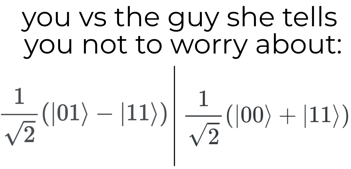
<p><img src="/assets/img/quantum_ent_worry_meme.png" alt="Worry Meme" title="worry_meme" /></p>

<p>Okay, we described multiple qubit states. You might scratch your head “Well, so what?”.</p>

<p>It turns out that we can have states that are not a product of individual qubit states! Consider the following state (read “ket phi plus”)</p>

\[\lvert \Phi^+ \rangle = \frac{1}{\sqrt{2}}(\lvert 00 \rangle + \lvert 11 \rangle)\]

<p>We can play a little with this state</p>

\[\lvert \Phi^+ \rangle = \alpha_b \cdot \alpha_a \lvert 00 \rangle + \alpha_b \cdot \beta_a \lvert 01 \rangle + \beta_b \cdot \alpha_a \lvert 10 \rangle + \beta_b \cdot \beta_a \lvert 11 \rangle \\
\frac{1}{\sqrt{2}}\lvert 00 \rangle - \frac{1}{\sqrt{2}}\lvert 11 \rangle = \alpha_b \cdot \alpha_a \lvert 00 \rangle + \alpha_b \cdot \beta_a \lvert 01 \rangle + \beta_b \cdot \alpha_a \lvert 10 \rangle + \beta_b \cdot \beta_a \lvert 11 \rangle \\
\alpha_b \cdot \alpha_a = \frac{1}{\sqrt{2}} \text{ (eq. 1)} \\
\alpha_b \cdot \beta_a = 0  \text{ (eq. 2)}\\
\beta_b \cdot \alpha_a = 0  \text{ (eq. 3)}\\
\beta_b \cdot \beta_a = -\frac{1}{\sqrt{2}}  \text{ (eq. 4)}\\\]

<p>Okay, so let us tackle this problem with basic equation-solving skills! If we look at equations 1 and 2, we can deduce that $\alpha_b \neq 0$, otherwise we could not satisfy equation 1. That implies that $\beta_a$ is $0$. Whew, that was close! But if we look at equation 4 now, we end in a ditch, because it cannot be satisfied with $beta_a = 0$. This short reasoning shows that we cannot represent the $\lvert \Phi^- \rangle$ state by simply combining states of two single qubits.</p>

<p>So how could we achieve that?</p>

<p>With the help of quantum logic gates, obviously! We know that we can achieve $\lvert -1 \rangle$ state. We are missing a gate that would have a $4 \times 4$ matrix that would map (for example ) $\lvert -1 \rangle$ to $\lvert \Phi^- \rangle$. That means solving $\lvert \Phi^- \rangle = M \cdot \lvert -1 \rangle$. Moreover, to meet the requirements of a quantum logic gate, we need to ensure that $M$ is <a href="https://en.wikipedia.org/wiki/Unitary_matrix">unitary</a>. With some tinkering, we can get to</p>

\[M = \begin{bmatrix} 
0 &amp; 1 &amp; 0 &amp; 0 \\
1 &amp; 0 &amp; 0 &amp; 0 \\
0 &amp; 0 &amp; 1 &amp; 0 \\
0 &amp; 0 &amp; 0 &amp; -1 \\
\end{bmatrix}\]

<p>To sum up, we started with two qubits in a <em>product state</em> pushed those qubits through a gate, and ended up in an <em>entangled state</em> that cannot be split into two qubits.</p>

<h2 id="why-do-we-even-need-entangled-states">Why do we even need entangled states?</h2>

<p>Okay, we described entangled qubit states. You might scratch your head “Well, so what?”.</p>

<p>Quantum algorithms you might read about leverage entanglement to propose solutions that are computationally faster than the fastest known “classical” algorithms. This is why we need to grasp the idea of the entangled state.</p>

<p>I do not know whether an entangled state is strictly necessary for a quantum algorithm to have a “quantum advantage”, but <a href="https://quantumcomputing.stackexchange.com/questions/28410/is-quantum-computer-without-entanglement-no-better-than-anything-classically-ach">there are voices</a> saying that it is necessary. On the other hand <a href="https://www.fuw.edu.pl/~szczytko/NT/materialy/9_QC/QCwithoutEntanglement.pdf">there are papers</a> showing that there is a possible quantum advantage even without the entangled state. My opinion - as a layman - is anything realizable and practically useful will need entanglement along the way.</p>]]></content><author><name>Piotr Lewandowski</name><email>piotr.w.lewandowski@gmail.com</email></author><category term="quantum computing" /><category term="qiskit introduction course" /><category term="quantum" /><category term="probability" /><category term="amplitude" /><category term="entangled state" /><summary type="html"><![CDATA[Step beyond classical computation]]></summary></entry><entry><title type="html">Bit, qubit, probability, amplitude, and H-gate</title><link href="https://plewandow.ski/quantum%20computing/qiskit%20introduction%20course/quantum-notes-1-amplitude/" rel="alternate" type="text/html" title="Bit, qubit, probability, amplitude, and H-gate" /><published>2022-11-17T00:00:00+01:00</published><updated>2022-11-17T00:00:00+01:00</updated><id>https://plewandow.ski/quantum%20computing/qiskit%20introduction%20course/quantum-notes-1-amplitude</id><content type="html" xml:base="https://plewandow.ski/quantum%20computing/qiskit%20introduction%20course/quantum-notes-1-amplitude/"><![CDATA[<h2 id="motivation-battleplan-and-requirements">Motivation, Battleplan, and Requirements</h2>

<p>After reading <a href="https://learn.qiskit.org/course/introduction/what-is-quantum#what-4-0">What is quantum?</a> I did not feel like I fully grasped the intuition behind the H-gate. In this post, I attempt to build such intuition on a high level (without diving too deep into the technical description). To do so, we will execute the following battle plan - we will describe bits, then qubits and amplitudes, then how amplitude relates to probability. Finally, we will tackle the boss-level concept of the H-gate.</p>

<p>I assume you are familiar (that does not mean being super proficient) with those concepts: <a href="https://en.wikipedia.org/wiki/Boolean_algebra#Basic_operations">basic Boolean logic</a>, <a href="https://en.wikipedia.org/wiki/Vector_(mathematics_and_physics)">vectors</a>, <a href="https://en.wikipedia.org/wiki/Matrix_(mathematics)">matrices</a>, <a href="https://en.wikipedia.org/wiki/Matrix_multiplication">matrix multiplication</a>, and <a href="https://en.wikipedia.org/wiki/Complex_number">complex numbers</a>.</p>

<h2 id="bits">Bits</h2>

<p>I really like the description of what bit is from <a href="https://en.wikipedia.org/wiki/Bit">Wiki</a>:</p>
<blockquote>
  <p>The bit is the most basic unit of information […]. The bit represents a logical state with one of two possible values.</p>
</blockquote>

<p>This short description works very well for me, especially after I took it apart. The highlights are <em>basic unit of information</em>, <em>state with two possible values</em>. If we think about what the minimal amount of information we can convey is that whether something <em>is</em> or <em>is not</em>. And that’s how I do interpret bits.</p>

<p>Please note that we did not describe how bits are <em>physically realized</em>. We described them as abstract objects. Bits can be realized in any physical thing that has two distinct states. For example with something as simple as a light switch with on and off positions. The core point is we do not really care about this, we just care about the properties of bits and what we can do with them as a perfect, mathematical object.</p>

<p>Of course bits, themselves are pretty boring. The action starts with logic gates! Logic gates are simply implementations of logical operations - think your ANDs, NOTs, ORs, and XORs.</p>

<p><em>NOT</em> is probably the simplest gate - it takes a bit and returns the inverse of it. For <code class="language-plaintext highlighter-rouge">0</code> (<em>is not</em>) it returns <code class="language-plaintext highlighter-rouge">1</code> (<em>is</em>). <em>AND</em> takes two bits and checks, whether both of them <em>are</em>. For <code class="language-plaintext highlighter-rouge">1</code> and <code class="language-plaintext highlighter-rouge">1</code>, it will return <code class="language-plaintext highlighter-rouge">1</code> and for every other input it would return <code class="language-plaintext highlighter-rouge">0</code>.</p>

<h2 id="qubits-and-amplitude">Qubits and amplitude</h2>

<p>First of all <em>qubits</em> are also (but not only) abstract, mathematical objects. What makes it easier for me to deal with them is to treat them as such - if I see a surprising qubit property, but can understand (or at least have intuition) about the math behind it - then I am all good.  I tell myself that “surprising properties of qubits are just consequence of math” to avoid mind-bending quantum effects which are so distinct from our day-to-day experience.</p>

<p>Just like a bit, a qubit also has two states, but instead of representing a logical state, it represents a quantum state. Now let us take jump head first and try to swim. Quantum state $\lvert \psi \rangle$ of a qubit can be defined as:</p>

\[\lvert \psi \rangle = \alpha \lvert 0 \rangle + \beta \lvert 1 \rangle; \alpha, \beta \in \mathbb{C} \text{ and } {\lvert \alpha \rvert}^2 + {\lvert \beta \rvert}^2 = 1\]

<p>Now let us take the equation above apart. First the $\lvert \text{something} \rangle$ notation - for our purposes it can just mean <em>quantum state</em>. If you want to dive deeper you should start reading up on <a href="https://en.wikipedia.org/wiki/Bra%E2%80%93ket_notation">Dirac notation</a>. With that $\lvert 0 \rangle$ is analogous to a $0$ state of a classic bit and $\lvert 1 \rangle$ to a classic bit with state $1$. What is important to know is that the aforementioned <em>quantum state</em> can be represented as a vector:</p>

\[\lvert 0 \rangle = \begin{pmatrix} 1 \\ 0 \end{pmatrix} \\
\lvert 1 \rangle = \begin{pmatrix} 0 \\ 1 \end{pmatrix} \\
\lvert \psi \rangle = \alpha \lvert 0 \rangle + \beta \lvert 1 \rangle = \alpha \begin{pmatrix} 1 \\ 0 \end{pmatrix} + \beta \begin{pmatrix} 0 \\ 1 \end{pmatrix} = \begin{pmatrix} \alpha \\ 0 \end{pmatrix} + \begin{pmatrix} 0 \\ \beta \end{pmatrix} = \begin{pmatrix} \alpha \\ \beta \end{pmatrix}\]

<p>Now let us tackle the $\alpha$ and $\beta$. As we can see above they describe how much state $\lvert \psi \rangle$ consists of $\lvert 0 \rangle$ and how much of $\lvert 1 \rangle$. Both $\alpha$ and $\beta$ are <em>probability amplitudes</em>. Probability amplitude is a complex number with the following property - <em>square 
modulus of probability amplitude equals probability of a particular outcome</em> (this is simplified, visit <a href="https://en.wikipedia.org/wiki/Probability_amplitude">Wiki</a> for more formal exposition).</p>

<p>Now we can interpret $\lvert \psi \rangle = \alpha \lvert 0 \rangle + \beta \lvert 1 \rangle$ as a state that has ${\lvert \alpha \rvert}^2$ probability of being $0$ and ${\lvert \beta \rvert}^2$ of being $1$! Remember that, when we will measure the state of a qubit we will see either $0$ or $1$, not some “in-between” state.</p>

<h2 id="quantum-logic-gates">Quantum logic gates</h2>

<p>With that, we can now attack quantum logic gates and H-gate. We know that quantum gates will take as an input a quantum state (at least one) and return another quantum state. If we define input and output quantum states as</p>

\[\lvert \psi_i \rangle = \begin{pmatrix} \alpha_i \\ \beta_i \end{pmatrix},
\lvert \psi_o \rangle = \begin{pmatrix} \alpha_o \\ \beta_o \end{pmatrix}\]

<p>then for a quantum logic gate to be expressive we would like to freely combine input values with the output ones, so we want</p>

\[\alpha_o = a \cdot \alpha_i + b \cdot \beta_i \\ 
\beta_o = c \cdot \alpha_i + d \cdot \beta_i\]

<p>If you recall your linear algebra course that is exactly how matrix multiplication works! So we can use our gate in the following ways</p>

\[\lvert \psi_o \rangle = \text{gate_matrix} \cdot \lvert \psi_i \rangle\]

<p>For a single qubit gate, we have the <em>gate matrix</em> needs to be $2 \times 2$</p>

\[\text{gate_matrix} = \begin{bmatrix} a &amp;&amp; b \\ c &amp;&amp; d \end{bmatrix}\]

<p>The output state needs to conform to the ${\lvert \alpha \rvert}^2 + {\lvert \beta \rvert}^2 = 1$. This is achieved by using <a href="https://en.wikipedia.org/wiki/Unitary_matrix">unitary matrices</a>.</p>

<p>Let us now look at the gate that would <em>inverse</em> the quantum state - mapping $0$ to $1$ and $1$ to $0$.</p>

\[\lvert 0 \rangle = \begin{pmatrix} 1 \\ 0 \end{pmatrix} = \begin{bmatrix} 0 &amp;&amp; 1 \\ 1 &amp;&amp; 0 \end{bmatrix} \cdot \begin{pmatrix} 0 \\ 1 \end{pmatrix} = \begin{bmatrix} 0 &amp;&amp; 1 \\ 1 &amp;&amp; 0 \end{bmatrix} \cdot \lvert 1 \rangle\]

<p>This quantum logic gate is called an <em>X-gate</em>. It is analogous to a NOT gate.</p>

<h2 id="h-gate">H-gate</h2>

<p>Finally, we can tackle the H-gate. Let us recall the properties of H-gate from the <a href="https://learn.qiskit.org/course/introduction/what-is-quantum#what-4-0">What is quantum?</a> section in the qiskit textbook.</p>

<ol>
  <li>Starting $\lvert 0 \rangle$ and $\lvert 1 \rangle$ we ended up with $0.5$ probability of observing $0$ and $0.5$ probability observing $1$. The output state of applying H-gate to $\lvert \psi \rangle$ would have following form - 
$\lvert \psi_H \rangle = \sqrt{\frac{1}{2}} \lvert 0 \rangle \pm \sqrt{\frac{1}{2}}$ $\lvert 1 \rangle$. The $\pm$ comes from the fact that if we want to get 0.5 probability by squaring a modulus of a complex number, we can do it from both $+\sqrt{\frac{1}{2}}$ and $-\sqrt{\frac{1}{2}}$.</li>
  <li>Applying H-gate twice takes us back to our initial state - $\lvert \psi_{HH} \rangle = \lvert \psi \rangle$</li>
</ol>

<p>Those two properties bring us to the following H-gate matrix (you can do the math on your own, it is not that hard!)</p>

\[H_{gate} = \frac{1}{\sqrt{2}} \begin{bmatrix} 1 &amp;&amp; 1 \\ 1 &amp;&amp; -1 \end{bmatrix}\]

<h3 id="notes-on-amplitude-as-a-vector">Notes on amplitude as a vector</h3>

<p>As amplitudes are complex numbers we can represent them using <a href="https://en.wikipedia.org/wiki/Polar_coordinate_system#Complex_numbers">polar coordinates</a>, with modulus becoming the length of vector formed between the origin point and any particular complex number. For me (on my current level of knowledge) thinking about amplitudes as vectors make things more “complete”. Then, for $\lvert 1 \rangle$ H-gate performs rotation of the amplitude vector (for the $\lvert 1 \rangle$ output).</p>

<h2 id="summary">Summary</h2>

<p>We described what bit is, then we went a level higher to describe qubit. We focused on the qubit complicated state which allowed us to describe quantum logic gates and finally define H-gate. I hope that this will help build your intuition and progress through the qiskit learning course!</p>]]></content><author><name>Piotr Lewandowski</name><email>piotr.w.lewandowski@gmail.com</email></author><category term="quantum computing" /><category term="qiskit introduction course" /><category term="quantum" /><category term="probability" /><category term="amplitude" /><category term="h-gate" /><summary type="html"><![CDATA[Qiskit introduction course notes #1]]></summary></entry><entry><title type="html">Typeclasses - FP Ladder 02</title><link href="https://plewandow.ski/scala/fp/fp-ladder/typeclass/typeclasses/" rel="alternate" type="text/html" title="Typeclasses - FP Ladder 02" /><published>2020-03-19T00:00:00+01:00</published><updated>2020-03-19T00:00:00+01:00</updated><id>https://plewandow.ski/scala/fp/fp-ladder/typeclass/typeclasses</id><content type="html" xml:base="https://plewandow.ski/scala/fp/fp-ladder/typeclass/typeclasses/"><![CDATA[<p>Wpis ten jest dość długi, ale zależy mi, żeby był <em>(względnie) kompletnym wstępem</em> do idei <em>typeclass</em> w Scali. Nie jest to koncept łatwy, ale jest niezbędny do wejścia powyżej poziomu podstawowego w Scali.</p>

<p>Polimorfizm jest jedną z podstawowych technik programowania w językach wysokiego poziomu. Jest bardzo popularny w językach obiektowych - i słusznie. Będąc wierny <em>jedynej słusznej drodze (JSD)</em>, czyli programowaniu funkcyjnemu, sądzę, że <em>polimorfizm o smaku ad-hoc</em> pozwala pisać w sposób naturalny kod, który jest bardziej modularny oraz uniwersalny.</p>

<h2 id="czym-jest-typ-klasa-klasa-typów">Czym jest typ, klasa, klasa typów?</h2>

<p>Zacznijmy od rozplątanie pojęć, które bywają używane zamiennie w kontekście tematu <em>typeclass</em>. Na końcu tej części powinno być jasne, czym ów twór jest.</p>
<ol>
  <li>Zbiór - w kontekście matematycznym - chyba najtrudniejsze do zdefiniowiania pojęcie. Jest to fundamentalne pojęcie <em>teorii mnogości</em>(Mnogość to inaczej zbiór, więc to po prostu teoria zbiorów). <em>Fundamentalne</em> oznacza tu, że jest to pojęcie tak pierwotne, że jest częściowo przyjmowane na zasadzie - “czym jest zbiór, każdy widzi” (to oczywiście zależy od podejścia do teorii mnogości jakie przyjmiemy, ale to wykracza poza nasze potrzeby). Intuicyjne jest to pewna kolekcja arbitralnie wybranych przez nas elementów.<br />
Ważniejsze są cechy zbioru - dany element może należeć do zbioru lub też nie, ale nie może przynależeć do niego dwukrotnie. Zbiór jest jednoznacznie wyznaczony przez jego elementy. To <em>tylko</em> tyle i <em>aż</em> tyle.</li>
  <li>Typ - w ujęciu programistycznym - znane nam dobrze <code class="language-plaintext highlighter-rouge">Int</code>, <code class="language-plaintext highlighter-rouge">String</code>, <code class="language-plaintext highlighter-rouge">List[T]</code>, czy też stworzone przez nas <code class="language-plaintext highlighter-rouge">class Animal</code>, <code class="language-plaintext highlighter-rouge">trait Money</code>, <code class="language-plaintext highlighter-rouge">object Earth</code>. Jest to cecha danych, która mówi kompilatorowi w jaki sposób chcemy użyć danych i na jakie operacje powinien nam na nich pozwolić. Zwróćmy uwagę na analogię pomiędzy zbiorem a typem, posłużmy się do tego funkcją:
    <div class="language-scala highlighter-rouge"><div class="highlight"><pre class="highlight"><code><table class="rouge-table"><tbody><tr><td class="rouge-gutter gl"><pre class="lineno">1
</pre></td><td class="rouge-code"><pre><span class="k">def</span> <span class="nf">isDivisableBy3</span><span class="o">(</span><span class="n">x</span><span class="k">:</span> <span class="kt">Int</span><span class="o">)</span><span class="k">:</span> <span class="kt">Boolean</span> <span class="o">=</span> <span class="n">x</span> <span class="o">%</span> <span class="mi">3</span> <span class="o">==</span> <span class="mi">0</span>
</pre></td></tr></tbody></table></code></pre></div>    </div>
    <p>Funkcja ta sprawdza, czy przekazany <code class="language-plaintext highlighter-rouge">Int</code> jest podzielny przez <code class="language-plaintext highlighter-rouge">3</code>. Informuje nas o to zwracając odpowiednią wartość <code class="language-plaintext highlighter-rouge">true</code> lub <code class="language-plaintext highlighter-rouge">false</code>. Spójrzmy na to jednak z małą matematyczną lupą. Zdefiniowaliśmy funkcję, która przypisuje elementom zbioru <code class="language-plaintext highlighter-rouge">Int</code> któryś z elementów zbioru <code class="language-plaintext highlighter-rouge">Boolean</code>. Tak więc wartości <code class="language-plaintext highlighter-rouge">true</code>, <code class="language-plaintext highlighter-rouge">false</code> należą do zbioru <code class="language-plaintext highlighter-rouge">Boolean</code> - stąd też ich typ. Analogicznie ze zbiorem <code class="language-plaintext highlighter-rouge">Int</code>, będącego skończonym podzbiorem liczb całkowitych.</p>
  </li>
  <li>Klasa - w ujęciu matematycznym - Pojęcie jest używane w matematyce, gdy mamy do czynienia z <em>wielością</em> (celowo nie zbiorem), który jest zbyt liczny i odrobinę zbyt zaskakujący, żeby go badać przy pomocy narzędzi teorii mnogości. Na nasze potrzeby wystarczy intuicja, mówiąca, że <em>klasa to grupa obiektów, która jest określona przez pewną wspólną własność</em>.</li>
  <li>Klasa - w ujęciu programistycznym - liczę na to, że czytelnik jest zaznajomiony z tym pojęciem. Ewentualną dygresją, którą warto dodać, że jest to pewne narzędzie, które służy nam do modelowania domeny problemu.</li>
  <li>Klasa typów - <em>typeclass</em> - Jest to połączenie konceptu klasy matematycznej z typem programistycznym. Więc mówiąc <em>typeclass</em> mamy na myśli pewną <em>grupę typów, które mają jakąś wspólną własność</em>. W praktyce przez wspólną własność zazwyczaj rozumiemy określoną na tych typach funkcję.</li>
</ol>

<p>Przykładem, który weźmiemy sobię pod lupę jest serializacja danych do formatu JSON. Naszym bardzo (a nawet bardzo, bardzo - nie bieżcie go za wzór przy modelowaniu czegokolwiek) uproszczonym punktem początkowym będzie</p>
<div class="language-scala highlighter-rouge"><div class="highlight"><pre class="highlight"><code><table class="rouge-table"><tbody><tr><td class="rouge-gutter gl"><pre class="lineno">1
2
3
4
5
6
7
</pre></td><td class="rouge-code"><pre><span class="k">case</span> <span class="k">class</span> <span class="nc">Account</span><span class="o">(</span><span class="n">id</span><span class="k">:</span> <span class="kt">String</span><span class="o">,</span> <span class="n">balance</span><span class="k">:</span> <span class="kt">BigDecimal</span><span class="o">)</span> <span class="o">{</span>
  <span class="k">def</span> <span class="nf">toJsonString</span><span class="k">:</span> <span class="kt">String</span> <span class="o">=</span> <span class="o">???</span> <span class="c1">// we do not care about implementation</span>
<span class="o">}</span>

<span class="k">case</span> <span class="k">class</span> <span class="nc">Dog</span><span class="o">(</span><span class="n">name</span><span class="k">:</span> <span class="kt">String</span><span class="o">,</span> <span class="n">breed</span><span class="k">:</span> <span class="kt">String</span><span class="o">,</span> <span class="n">weight</span><span class="k">:</span> <span class="kt">Int</span><span class="o">)</span> <span class="o">{</span>
  <span class="k">def</span> <span class="nf">toJsonString</span><span class="k">:</span> <span class="kt">String</span> <span class="o">=</span> <span class="o">???</span> <span class="c1">// we do not care about implementation</span>
<span class="o">}</span>
</pre></td></tr></tbody></table></code></pre></div></div>
<p>Bez żadnego naciągactwa możemy powiedzieć, że chcielibyśmy wprowadzić pewną klasę typów, która pozwoli nam mówić o klasach, które możemy serializować do formatu JSON.</p>

<h2 id="seperacja-zachowania-od-danych">Seperacja zachowania od danych</h2>

<p>Zanim jednak wypłyniemy na wzburzone morza <em>typeclass</em> o modularności. Jestem zwolennikiem seperacji <em>zachowania</em> danych od ich <em>definicji</em>. Programiści (w tym ja!) często - przypadkiem - doprowadzają często do splątania tych dwóch rzeczy, a to w efekcie zmniejsza modularność naszego kodu. Zmniejszenie modularności powoduje, że nasz kod jest ciężej używać w różnych, niezależnych od siebie miejscach, ciężej go testować i ogólnie zwiększa stopień “kaszanowatości” rozwiązania. Wyobraźmy sobie nie najlepiej zamodelowaną klasę:</p>
<div class="language-scala highlighter-rouge"><div class="highlight"><pre class="highlight"><code><table class="rouge-table"><tbody><tr><td class="rouge-gutter gl"><pre class="lineno">1
2
3
4
5
6
7
</pre></td><td class="rouge-code"><pre><span class="k">case</span> <span class="k">class</span> <span class="nc">Account</span><span class="o">(</span><span class="n">id</span><span class="k">:</span> <span class="kt">String</span><span class="o">,</span> <span class="n">balance</span><span class="k">:</span> <span class="kt">BigDecimal</span><span class="o">)</span> <span class="o">{</span>
  <span class="k">def</span> <span class="nf">toJsonString</span><span class="k">:</span> <span class="kt">String</span> <span class="o">=</span> <span class="o">???</span> <span class="c1">// we do not care about implementation</span>

  <span class="k">def</span> <span class="nf">closeAccount</span><span class="k">:</span> <span class="kt">ClosingResult</span> <span class="o">=</span> <span class="o">???</span> 

  <span class="k">def</span> <span class="nf">buyDog</span><span class="o">(</span><span class="n">dog</span><span class="k">:</span> <span class="kt">Dog</span><span class="o">,</span> <span class="n">money</span><span class="k">:</span> <span class="kt">BigDecimal</span><span class="o">)</span><span class="k">:</span> <span class="kt">Dog</span> <span class="o">=</span> <span class="o">???</span>
<span class="o">}</span>
</pre></td></tr></tbody></table></code></pre></div></div>
<p>Mamy do czynienia tutaj z pomieszaniem z poplątaniem. Moduł naszej aplikacji odpowiedzialny za zamykanie i autoryzacje kont teraz jest pośrednio zależny od <code class="language-plaintext highlighter-rouge">buyDog</code> - jeżeli zmienia się definicja tej funkcji, wszyscy użytkownicy tej klasy muszą zostać o tym poinformowani. W mojej ocenie co jest jeszcze gorsze dajemy możliwości kupowania psów modułowi autoryzacyjnemy oraz zamykania konta modułowi odpowiedzialnymi za sprzedaż piesków! Pozwól danym być danymi, nie zmuszaj ich do niewolniczej pracy.</p>

<p>Podejście to jest oczywiście efektem dobrych praktyk programistycznych (single responsibility principle, seperation of concerns i innych).</p>

<p>Co to nam mówi o “serializowalnym” <code class="language-plaintext highlighter-rouge">Account</code> i <code class="language-plaintext highlighter-rouge">Dog</code>? Nie powinniśmy plątać definicji serializacji i definicji danych.</p>

<h2 id="do-rzeczy---jak-ten-typeclass-wygląda-w-scali">Do rzeczy - jak ten <em>typeclass</em> wygląda w Scali?</h2>

<p>Żeby zdefiniować klasę typów, które będą mogły być serializowane do JSON możemy zacząć od definicji <code class="language-plaintext highlighter-rouge">trait</code>:</p>
<div class="language-scala highlighter-rouge"><div class="highlight"><pre class="highlight"><code><table class="rouge-table"><tbody><tr><td class="rouge-gutter gl"><pre class="lineno">1
2
3
</pre></td><td class="rouge-code"><pre><span class="k">trait</span> <span class="nc">JsonEncodable</span><span class="o">[</span><span class="kt">A</span><span class="o">]</span> <span class="o">{</span>
   <span class="k">def</span> <span class="nf">toJsonString</span><span class="o">(</span><span class="n">a</span><span class="k">:</span> <span class="kt">A</span><span class="o">)</span><span class="k">:</span> <span class="kt">String</span>
<span class="o">}</span>
</pre></td></tr></tbody></table></code></pre></div></div>
<p>A cóż to za parametr <code class="language-plaintext highlighter-rouge">A</code>? Naszą klasą typów jest <code class="language-plaintext highlighter-rouge">JsonEncodable</code> natomiast z punktu widzenia języka programowania będziemy musieli w jakiś sposób pokazać, że dany typ przynależy do klasy <code class="language-plaintext highlighter-rouge">JsonEncodable</code> - odbędzie się to przez implementację <code class="language-plaintext highlighter-rouge">JsonEncodable</code>:</p>

<div class="language-scala highlighter-rouge"><div class="highlight"><pre class="highlight"><code><table class="rouge-table"><tbody><tr><td class="rouge-gutter gl"><pre class="lineno">1
2
3
4
5
6
</pre></td><td class="rouge-code"><pre><span class="k">object</span> <span class="nc">Account</span> <span class="o">{</span>
  <span class="k">implicit</span> <span class="k">val</span> <span class="nv">enc</span><span class="k">:</span> <span class="kt">JsonEncodable</span><span class="o">[</span><span class="kt">Account</span><span class="o">]</span> <span class="k">=</span> <span class="k">new</span> <span class="nc">JsonEncodable</span> <span class="o">{</span>
    <span class="k">override</span> <span class="k">def</span> <span class="nf">toJsonString</span><span class="o">(</span><span class="n">account</span><span class="k">:</span> <span class="kt">Account</span><span class="o">)</span><span class="k">:</span> <span class="kt">String</span> <span class="o">=</span> <span class="o">???</span> <span class="c1">// we do not care about implementation.</span>
  <span class="o">}</span>
<span class="o">}</span>

</pre></td></tr></tbody></table></code></pre></div></div>
<p>Teraz żeby zserializować obiekt Account możemy napisać:</p>

<div class="language-scala highlighter-rouge"><div class="highlight"><pre class="highlight"><code><table class="rouge-table"><tbody><tr><td class="rouge-gutter gl"><pre class="lineno">1
2
</pre></td><td class="rouge-code"><pre><span class="k">val</span> <span class="nv">account</span><span class="k">:</span> <span class="kt">Account</span> <span class="o">=</span> <span class="nc">Account</span><span class="o">(</span><span class="s">"id"</span><span class="o">,</span> <span class="mi">100</span><span class="o">)</span>
<span class="k">val</span> <span class="nv">jsonString</span><span class="k">:</span> <span class="kt">String</span> <span class="o">=</span> <span class="nv">Account</span><span class="o">.</span><span class="py">enc</span><span class="o">.</span><span class="py">toJsonString</span><span class="o">(</span><span class="n">account</span><span class="o">)</span>
</pre></td></tr></tbody></table></code></pre></div></div>

<p>Możemy pozwolić sobie również tworzenie generycznych funkcji:</p>
<div class="language-scala highlighter-rouge"><div class="highlight"><pre class="highlight"><code><table class="rouge-table"><tbody><tr><td class="rouge-gutter gl"><pre class="lineno">1
</pre></td><td class="rouge-code"><pre><span class="k">def</span> <span class="nf">genericToJsonString</span><span class="o">[</span><span class="kt">A</span><span class="o">](</span><span class="n">a</span><span class="k">:</span> <span class="kt">A</span><span class="o">,</span> <span class="n">ev</span><span class="k">:</span> <span class="kt">JsonEncodable</span><span class="o">[</span><span class="kt">A</span><span class="o">])</span> <span class="k">=</span> <span class="nv">ev</span><span class="o">.</span><span class="py">toJsonString</span><span class="o">(</span><span class="n">a</span><span class="o">)</span>
</pre></td></tr></tbody></table></code></pre></div></div>

<h3 id="po-co-to-wszystko">Po co to wszystko?</h3>

<p>Pierwszą zaletą jest fakt odseperowania zachowania od definicji danych. Kolejną jest przekazanie części pracy kompilatorowi, funkcja <code class="language-plaintext highlighter-rouge">genericToJsonString[A]</code> wymaga zaimplementowanego <code class="language-plaintext highlighter-rouge">ev: JsonEncodable[A]</code> (<code class="language-plaintext highlighter-rouge">ev</code> jest skrótem od <em>evidence</em>).<br />
Drugą jest możliwość deklarowania różnych implementacji dla kompletnie różnych typów, które same w sobie nie muszą być ze sobą w żaden sposób związane (musi istnieć odpowiednia implementacja <code class="language-plaintext highlighter-rouge">JsonEncodable</code> dla typu <code class="language-plaintext highlighter-rouge">A</code>) - nazywamy to <a href="https://en.wikipedia.org/wiki/Ad_hoc_polymorphism"><em>ad-hoc polymorphism</em></a>. Zwróć uwagę na fakt, że w żaden sposób nie narzuciliśmy ograniczeń na typ <code class="language-plaintext highlighter-rouge">A</code>.
Trzecią zaletą możliwość rozszerzanie funkcjonalności typów bez dostępu do ich kodu źrodłowego (<code class="language-plaintext highlighter-rouge">JsonEncodable[Account]</code> możemy zaimplementować bez dostępu do kodu źrodłowego <code class="language-plaintext highlighter-rouge">Account</code>).</p>

<h3 id="no-strasznie-to-brzydkie">No strasznie to brzydkie</h3>

<p>Faktycznie zapis <code class="language-plaintext highlighter-rouge">def genericToJsonString[A](a: A, ev: JsonEncodable[A]) = ev.toJsonString(a)</code> wygląda dość ociężale. Scala jednak pozwala na kilka uproszczeń.</p>
<div class="language-scala highlighter-rouge"><div class="highlight"><pre class="highlight"><code><table class="rouge-table"><tbody><tr><td class="rouge-gutter gl"><pre class="lineno">1
</pre></td><td class="rouge-code"><pre><span class="k">def</span> <span class="nf">genericToJsonString</span><span class="o">[</span><span class="kt">A</span><span class="o">](</span><span class="n">a</span><span class="k">:</span> <span class="kt">A</span><span class="o">)(</span><span class="k">implicit</span> <span class="n">ev</span><span class="k">:</span> <span class="kt">JsonEncodable</span><span class="o">[</span><span class="kt">A</span><span class="o">])</span> <span class="k">=</span> <span class="nv">ev</span><span class="o">.</span><span class="py">toJsonString</span><span class="o">(</span><span class="n">a</span><span class="o">)</span>
</pre></td></tr></tbody></table></code></pre></div></div>
<p>Wtedy serializacja typu <code class="language-plaintext highlighter-rouge">Account</code> będzie uproszczona - tak długo jak w zasięgu kompilatora będzie <code class="language-plaintext highlighter-rouge">implicit val enc: JsonEncodable[A]</code>. Obecnie zdeklarowaliśmy go w companion object <code class="language-plaintext highlighter-rouge">Account</code>, więc zawsze gdy zaimportujemy <code class="language-plaintext highlighter-rouge">Account</code> pojawi się nasz encoder, co pozwoli nam napisać:</p>
<div class="language-scala highlighter-rouge"><div class="highlight"><pre class="highlight"><code><table class="rouge-table"><tbody><tr><td class="rouge-gutter gl"><pre class="lineno">1
2
</pre></td><td class="rouge-code"><pre><span class="k">val</span> <span class="nv">account</span><span class="k">:</span> <span class="kt">Account</span> <span class="o">=</span> <span class="nc">Account</span><span class="o">(</span><span class="s">"id"</span><span class="o">,</span> <span class="mi">100</span><span class="o">)</span>
<span class="k">val</span> <span class="nv">jsonString</span><span class="k">:</span> <span class="kt">String</span> <span class="o">=</span> <span class="nf">genericToJsonString</span><span class="o">(</span><span class="n">account</span><span class="o">)</span>
</pre></td></tr></tbody></table></code></pre></div></div>

<p>Kolejnym uproszczeniem jest następujący zapis:</p>
<div class="language-scala highlighter-rouge"><div class="highlight"><pre class="highlight"><code><table class="rouge-table"><tbody><tr><td class="rouge-gutter gl"><pre class="lineno">1
</pre></td><td class="rouge-code"><pre><span class="k">def</span> <span class="nf">genericToJsonString</span><span class="o">[</span><span class="kt">A:</span> <span class="kt">JsonEncodable</span><span class="o">](</span><span class="n">a</span><span class="k">:</span> <span class="kt">A</span><span class="o">)</span> <span class="k">=</span> <span class="nc">JsonEncodable</span><span class="o">[</span><span class="kt">A</span><span class="o">].</span><span class="py">toJsonString</span><span class="o">(</span><span class="n">a</span><span class="o">)</span>
</pre></td></tr></tbody></table></code></pre></div></div>
<p>Żeby jednak kompilator był zadowolony (zadowolony kompilator to sprawa istotna) musimy stworzyć companion object do <code class="language-plaintext highlighter-rouge">JsonEncodable</code>:</p>
<div class="language-scala highlighter-rouge"><div class="highlight"><pre class="highlight"><code><table class="rouge-table"><tbody><tr><td class="rouge-gutter gl"><pre class="lineno">1
2
3
</pre></td><td class="rouge-code"><pre><span class="k">object</span> <span class="nc">JsonEncodable</span> <span class="o">{</span>
  <span class="k">def</span> <span class="nf">apply</span><span class="o">[</span><span class="kt">A</span><span class="o">](</span><span class="k">implicit</span> <span class="n">ev</span><span class="k">:</span> <span class="kt">JsonEncodable</span><span class="o">[</span><span class="kt">A</span><span class="o">])</span><span class="k">:</span> <span class="kt">JsonEncodable</span><span class="o">[</span><span class="kt">A</span><span class="o">]</span> <span class="k">=</span> <span class="n">ev</span>
<span class="o">}</span>
</pre></td></tr></tbody></table></code></pre></div></div>
<p>To pozwoli nam również na zapis:</p>
<div class="language-scala highlighter-rouge"><div class="highlight"><pre class="highlight"><code><table class="rouge-table"><tbody><tr><td class="rouge-gutter gl"><pre class="lineno">1
2
</pre></td><td class="rouge-code"><pre><span class="k">val</span> <span class="nv">account</span><span class="k">:</span> <span class="kt">Account</span> <span class="o">=</span> <span class="nc">Account</span><span class="o">(</span><span class="s">"id"</span><span class="o">,</span> <span class="mi">100</span><span class="o">)</span>
<span class="k">val</span> <span class="nv">jsonString</span><span class="k">:</span> <span class="kt">String</span> <span class="o">=</span> <span class="nf">genericToJsonString</span><span class="o">(</span><span class="n">account</span><span class="o">)</span>
</pre></td></tr></tbody></table></code></pre></div></div>
<p>Alterantywnie bez deklaracji companion object możemy pokusić się o takie sformułowanie:</p>
<div class="language-scala highlighter-rouge"><div class="highlight"><pre class="highlight"><code><table class="rouge-table"><tbody><tr><td class="rouge-gutter gl"><pre class="lineno">1
</pre></td><td class="rouge-code"><pre><span class="k">def</span> <span class="nf">genericToJsonString</span><span class="o">[</span><span class="kt">A:</span> <span class="kt">JsonEncodable</span><span class="o">](</span><span class="n">a</span><span class="k">:</span> <span class="kt">A</span><span class="o">)</span> <span class="k">=</span> <span class="n">implicitly</span><span class="o">[</span><span class="kt">JsonEncodable</span><span class="o">[</span><span class="kt">A</span><span class="o">]].</span><span class="py">toJsonString</span><span class="o">(</span><span class="n">a</span><span class="o">)</span>
</pre></td></tr></tbody></table></code></pre></div></div>
<p>Można (i należy) dalej “upiększać” przy pomocy <em>interface syntax</em> lub <em>interface object</em>, o których warto przeczytać <a href="https://alvinalexander.com/scala/fp-book/type-classes-101-introduction">tu</a></p>

<h3 id="podsumowanie-implementacji">Podsumowanie implementacji</h3>

<p>Żeby zaimplementować <em>typeclass</em> musimy zrobić przynajmniej poniższe dwie rzeczy:</p>
<ol>
  <li>Zdefiniować <em>typeclass</em>-ę jako generyczny (sparametryzowany przynajmniej przez jeden typ) <code class="language-plaintext highlighter-rouge">trait</code>, na przykład <code class="language-plaintext highlighter-rouge">JsonEncodable[A]</code>.</li>
  <li>Przynajmniej jedną implementację powyższej <em>typeclass</em>-y - w naszym wypadku była to <code class="language-plaintext highlighter-rouge">implicit val enc: JsonEncodable[Account] = ...</code>.</li>
</ol>

<h2 id="podsumowanie">Podsumowanie</h2>

<p>Mam nadzieję, że ten artykuł przybliżył Wam koncept <em>typeclass</em>-y. Jest to tylko wstęp, więc nie miej sobie za złe, jeżeli nie od razu widzisz zastosowania tej techniki. Postaram się to zmienić w kolejnych wpisach. Jest to jednak niezbędna widza, jeżeli chce się wejść na odrobinę wyższy poziom w Scali niż użycie <code class="language-plaintext highlighter-rouge">map</code> i <code class="language-plaintext highlighter-rouge">filter</code>.</p>]]></content><author><name>Piotr Lewandowski</name><email>piotr.w.lewandowski@gmail.com</email></author><category term="scala" /><category term="fp" /><category term="fp-ladder" /><category term="typeclass" /><summary type="html"><![CDATA[Twoja furtka do uzależniania od programowania funkcyjnego]]></summary></entry><entry><title type="html">Immutable Data - FP Ladder 01</title><link href="https://plewandow.ski/scala/fp/fp-ladder/immutable-data/" rel="alternate" type="text/html" title="Immutable Data - FP Ladder 01" /><published>2020-03-15T00:00:00+01:00</published><updated>2020-03-15T00:00:00+01:00</updated><id>https://plewandow.ski/scala/fp/fp-ladder/immutable-data</id><content type="html" xml:base="https://plewandow.ski/scala/fp/fp-ladder/immutable-data/"><![CDATA[<p>W pracy mam przyjemność pomagać przy rekrutacji, co czasami wiąże się ze sprawdzeniem kawałka kodu napisanego w Scali. Jakość tych rozwiązań jest - oczywiście - na różnym poziomie, ale często przewijają się podobne błędy, szczególnie u osób zaczynających przygodę ze Scalą/FP. Jednym z takich błędów jest używanie <em>zmiennych</em> (<em>variables</em>) oraz <em>zmiennych struktur danych</em> (<em>mutable data structures</em>). W tym wpisie zaprezentuję naturalną dla Scali (i innych typowanych języków pozwalających na programowanie funkcyjne) alternatywę.</p>

<h2 id="zmienna-i-stała">Zmienna i stała</h2>

<p>Używając Scali możemy określić wartość na dwa podstawowe sposoby <code class="language-plaintext highlighter-rouge">var</code> oraz <code class="language-plaintext highlighter-rouge">val</code>. <code class="language-plaintext highlighter-rouge">var</code> jest skrótem od angielskiego <code class="language-plaintext highlighter-rouge">variable</code>, dosłownie oznaczającą <em>zmienną</em>, <code class="language-plaintext highlighter-rouge">val</code> natomiast jest skrótem od <code class="language-plaintext highlighter-rouge">value</code> oznaczającego <em>wartość</em>. Zanim przejdziemy dalej, sądzę że należy rozprawić się z pewnym splątaniem tych pojęć.</p>
<ol>
  <li>W Scali, kiedy mówię o zmiennej mogę mieć na myśli zarówno <code class="language-plaintext highlighter-rouge">var x: Int</code> i <code class="language-plaintext highlighter-rouge">val x: Int</code>, a to nie pomaga. W praktyce, w związku z tym, że praktycznie nigdy nie używam <code class="language-plaintext highlighter-rouge">var</code> - mam na myśli <code class="language-plaintext highlighter-rouge">val</code>. Podobnie jest w innych językach typowanych, np. w Javie zmienną nazwę zarówno <code class="language-plaintext highlighter-rouge">int x</code> jak i <code class="language-plaintext highlighter-rouge">final int x</code>.</li>
  <li>W matematyce zmienna oznacza zazwyczaj wielkość, która może przyjmować wartości z określonego zbioru. Zmienną można <em>ustalić</em>, czyli określić konkretną wartość i już się jej trzymać - nazwiemy wtedy ją stałą.</li>
</ol>

<p>Warto zwrócić uwagę na pewną analogię pomiędzy tymi dwoma konstruktami, szczególnie na określenie <em>typu</em> w Scali oraz idee <em>zbioru</em> w matematyce.</p>

<h3 id="co-to-za-różnica">Co to za różnica?</h3>

<p>Słuszne pytanie! Zobaczmy więc jak zachowa się Scala, kiedy będziemy chcieli nadpisać wartość <code class="language-plaintext highlighter-rouge">var</code> oraz <code class="language-plaintext highlighter-rouge">val</code>.</p>
<div class="language-scala highlighter-rouge"><div class="highlight"><pre class="highlight"><code><table class="rouge-table"><tbody><tr><td class="rouge-gutter gl"><pre class="lineno">1
2
3
4
5
6
7
8
9
10
11
12
</pre></td><td class="rouge-code"><pre><span class="n">scala</span><span class="o">&gt;</span> <span class="k">var</span> <span class="n">x</span> <span class="k">=</span> <span class="mi">3</span>
<span class="n">x</span><span class="k">:</span> <span class="kt">Int</span> <span class="o">=</span> <span class="mi">3</span>

<span class="n">scala</span><span class="o">&gt;</span> <span class="n">x</span> <span class="k">=</span> <span class="mi">4</span>
<span class="n">x</span><span class="k">:</span> <span class="kt">Int</span> <span class="o">=</span> <span class="mi">4</span>

<span class="n">scala</span><span class="o">&gt;</span> <span class="k">val</span> <span class="nv">y</span> <span class="k">=</span> <span class="mi">3</span>
<span class="n">y</span><span class="k">:</span> <span class="kt">Int</span> <span class="o">=</span> <span class="mi">3</span>

<span class="n">scala</span><span class="o">&gt;</span> <span class="n">y</span> <span class="k">=</span> <span class="mi">5</span>
<span class="o">&lt;</span><span class="n">console</span><span class="k">&gt;:</span><span class="mi">12</span><span class="k">:</span> <span class="kt">error:</span> <span class="kt">reassignment</span> <span class="kt">to</span> <span class="kt">val</span>
       <span class="n">y</span> <span class="k">=</span> <span class="mi">5</span>
</pre></td></tr></tbody></table></code></pre></div></div>
<p>Okazuje się, że do <code class="language-plaintext highlighter-rouge">val</code> nie można ponownie przypisać wartości. Wydaje mi się, że zasadą, której należy się trzymać jest: <strong>Używaj tylko <code class="language-plaintext highlighter-rouge">val</code>, chyba że bardzo dobrze wiesz co robisz</strong>. Jest to podejście, które pozwoli szybciej wdrożyć się w <em>jedyną słuszą drogę (JSD)</em>, tj. programowanie funkcyjne. W mojej ocenie, nie korzystanie z narzędzi jakie Scala daje, tak by sprawnie pisać funkcyjnie jest powodem, żeby w ogóle ze Scali zrezygnować.</p>

<p>Oczywiście dobrze byłoby uzasadnić pogląd wyższości <code class="language-plaintext highlighter-rouge">val</code> nad <code class="language-plaintext highlighter-rouge">var</code>. W mojej ocenie kluczową zaletą jest <em>odciążenie mózgu</em>. Istnieje duże prawdopodobieństwo, że jest to spowodowane moimi umiarkowanymi mocami intelektualnymi. Zawsze byłem pełen podziwu dla osób, które są w stanie spamiętać, gdzie i kiedy każdy konkretny <code class="language-plaintext highlighter-rouge">var</code> się zmienia. Pamiętają też, żeby pilnować te wartości w środowisku wielowątkowym. Być może część funkcjonalności jest poprawnie oddelegowana do innej metody, która oddelegowuje gdzieś dalej, a oni wciąż pamiętają każdą zmianę. Ja niestety takich talentów nie posiadam, więc <em>uproszczenie</em> i <em>usystematyzowanie</em> myślenia o kodzie jest dla mnie wartościowe.</p>

<p>Możliwość <em>metodycznego</em> i <em>systematycznego</em> myślenia o kodzie jest dla mnie ważna i zwięszka zaufanie do tego co piszę ja oraz osoby, z którymi pracuję. Czytając wtedy kod, wiem, że nie ma gdzieś ukrytej wartości, która może - zazwyczaj w nietrywialnej sytuacji brzegowej - wporwadzić w osłupienie i skierać na nieprzetarte szlaki z wiernym debuggerem.</p>

<h2 id="co-ze-strukturami-danych">Co ze strukturami danych?</h2>

<p>Jeżeli takie zalety mają pojedyncze zmienne, to chicelibyśmy je generalizować na struktury danych. Na szczęście, rzeczywiście tak jest. W obrębie tego wpisu <em>struktury danych</em> rozumiem głównie klasy tworzone przez programistów, chociaż przenosi się to na “klasycznie” rozumiane struktury danych takie jak listy, słowniki, czy drzewa. W tym wypadku zazwyczaj w celach optymalizacyjnych implementacje zawierają jakiś stan, który jednak nie powinien wyciekać do użytkownika API takiej struktury.</p>

<p>Wróćmy do tworzonych przez nas klas oraz typów. Rozważmy uproszczony przykład konta bankowego, które posiada swój numer oraz stan dostępnych środków:</p>
<div class="language-plaintext highlighter-rouge"><div class="highlight"><pre class="highlight"><code><table class="rouge-table"><tbody><tr><td class="rouge-gutter gl"><pre class="lineno">1
</pre></td><td class="rouge-code"><pre>case class Account(var id: String, var balance: BigDecimal)
</pre></td></tr></tbody></table></code></pre></div></div>
<p>Jeżeli nawet odrobinę nie boli Cię widok takiej deklaracji, to powinien zacząć. Użycie <code class="language-plaintext highlighter-rouge">var</code> do określenia <code class="language-plaintext highlighter-rouge">id</code> jest zastanawiające niezależnie od tego z jakiej perspektywy patrzymy na nasz problem. Konto ma swój unikalny identyfikator i po utworzeniu nie powinniśmy móc go zmieniać.</p>

<p>Można natomiast próbować argumentować użycie <code class="language-plaintext highlighter-rouge">var balance: BigDecimal</code>. Przecież jak dostaję wypłatę, to nie mam nowego konta z wypłatą, lecz jest to <em>to samo konto, którego stan jest powiększony o kwotę wypłaty</em>. Ciężko się z tym nie zgodzić. Należy jednak pamiętać, że nie mamy obowiązku modelować świata w sposób identyczny, mamy tylko przedstawić jego reprezentację. Część osób zaznajomionych z DDD może powiedzieć, że <code class="language-plaintext highlighter-rouge">Account</code> to typowy przykład <em>entity</em> i związku z tym <code class="language-plaintext highlighter-rouge">balance</code> należy do pól, które mogą się zmieniać. W mojej ocenie jest to nadużycie koncepcji <em>entity</em> wewnątrz języka programowania i nie używanie poprawnie jego narzędzi, które nam dostarcza. Oczywiście nie podważam tutaj ani istotności DDD, ani <em>entity</em> przy modelowaniu domeny, po prostu nie wszystko należy przenosić dosłownie.</p>

<p>Konto po zwiększeniu kwoty nie staje się innym kontem. Jednak z punktu widzenia naszego kodu lepiej będzie, gdy wszystkie pola będą ustalone w momencie tworzenia, a do aktualizacji pól będziemy albo używać odpowienich metod, które będą zwracać <em>kopię obiektu z zaktualizowanymi wartościami</em>. W Scali każda <code class="language-plaintext highlighter-rouge">case class</code>a - a to właśnie ich powinniśmy używać do modelowania danych - ma metodę <code class="language-plaintext highlighter-rouge">copy</code>, która pozwala wygodnie zaktualizować wartość (są oczywiście jeszcze <code class="language-plaintext highlighter-rouge">lenses</code>, ale to podejście i temat przedyskutuję w oddzielnym wpisie). Poprawnie zamodelowana klasa <code class="language-plaintext highlighter-rouge">Account</code> i aktualizacja jej stanu powinna wyglądać następująco:</p>
<div class="language-scala highlighter-rouge"><div class="highlight"><pre class="highlight"><code><table class="rouge-table"><tbody><tr><td class="rouge-gutter gl"><pre class="lineno">1
2
3
4
5
6
7
8
</pre></td><td class="rouge-code"><pre><span class="n">scala</span><span class="o">&gt;</span> <span class="k">case</span> <span class="k">class</span> <span class="nc">Account</span><span class="o">(</span><span class="n">id</span><span class="k">:</span> <span class="kt">String</span><span class="o">,</span> <span class="n">balance</span><span class="k">:</span> <span class="kt">BigDecimal</span><span class="o">)</span>
<span class="n">defined</span> <span class="k">class</span> <span class="nc">Account</span>

<span class="n">scala</span><span class="o">&gt;</span> <span class="k">val</span> <span class="nv">acc</span> <span class="k">=</span> <span class="nc">Account</span><span class="o">(</span><span class="s">"id1"</span><span class="o">,</span> <span class="mi">0</span><span class="o">)</span>
<span class="n">acc</span><span class="k">:</span> <span class="kt">Account</span> <span class="o">=</span> <span class="nc">Account</span><span class="o">(</span><span class="n">id1</span><span class="o">,</span><span class="mi">0</span><span class="o">)</span>

<span class="n">scala</span><span class="o">&gt;</span> <span class="k">val</span> <span class="nv">accAfterPayday</span> <span class="k">=</span> <span class="nv">acc</span><span class="o">.</span><span class="py">copy</span><span class="o">(</span><span class="n">balance</span> <span class="k">=</span> <span class="nv">acc</span><span class="o">.</span><span class="py">balance</span> <span class="o">+</span> <span class="mi">100</span><span class="o">)</span>
<span class="n">accAfterPayday</span><span class="k">:</span> <span class="kt">Account</span> <span class="o">=</span> <span class="nc">Account</span><span class="o">(</span><span class="n">id1</span><span class="o">,</span><span class="mi">100</span><span class="o">)</span>
</pre></td></tr></tbody></table></code></pre></div></div>
<p>Zwróćmy uwagę, że w wypadku pominięcia słowa <code class="language-plaintext highlighter-rouge">var</code> Scala automatycznie uznaje pola klasy za niezmienne. <em>Zupełnie jakby chciała nam coś powiedzieć</em>. Oczywiście używanie <code class="language-plaintext highlighter-rouge">copy</code> może wydawać się dość siermiężne i należy używać odpowiednich technik - jak definiowanie dobrze nazwanych funkcji - by kod był siermiężny odrobinę mniej. Zasada, którą możemy wyciągnąć, mówi <strong>Używaj tylko niezmiennych struktur danych, chyba, że masz bardzo dobry powód by było inaczej</strong>. Z punktu widzenia użytkownika Twojej klasy - najlepiej, żeby API wyglądało jednak jakby było zupełnie <em>immutable</em>.</p>

<h2 id="podsumowanie">Podsumowanie</h2>

<p>Temat ten dla kogoś, kto pracował ze Scalą jest oczywiście zupełnie podstawowy. Widzę jednak, że osoby przychodzące ze świata javascriptu, php i innych języków często właśnie w taki sposób próbują rozwiązywać problemy. Trzymanie się dwóch wytłuszczonych “zasad”, które przytoczyłem pozwoli na pisanie kodu, który będzie odrobinę łatwiejszy w utrzymaniu, czytelniejszy oraz - jeżeli dopiero zaczynasz przygodę ze Scalą/FP - zadba o szybsze postępy i wykluczy pewne, zazwyczaj niezdrowe, nawyki.</p>]]></content><author><name>Piotr Lewandowski</name><email>piotr.w.lewandowski@gmail.com</email></author><category term="scala" /><category term="fp" /><category term="fp-ladder" /><summary type="html"><![CDATA[Zmiana nie zawsze jest dobra]]></summary></entry><entry><title type="html">Basics of Extreme Learning Machines</title><link href="https://plewandow.ski/elm/machine%20learning/neural%20networks/elm-basics/" rel="alternate" type="text/html" title="Basics of Extreme Learning Machines" /><published>2019-02-13T00:00:00+01:00</published><updated>2019-02-13T00:00:00+01:00</updated><id>https://plewandow.ski/elm/machine%20learning/neural%20networks/elm-basics</id><content type="html" xml:base="https://plewandow.ski/elm/machine%20learning/neural%20networks/elm-basics/"><![CDATA[<blockquote>
  <p>I based my post on <a href="http://axon.cs.byu.edu/~martinez/classes/678/Presentations/Yao.pdf">Extreme learning machine: Theory and applications, by Guang-Bin Huang, Qin-Yu Zhu, Chee-Kheong Siew</a>. That means that we will focus on neural networks with one hidden layer. Further advances have been made - for example using multiple hidden layers. If you are interested in that, you can visit <a href="http://www.ntu.edu.sg/home/egbhuang/">this site</a>. It is definitely worth it.</p>
</blockquote>

<h2 id="what-is-extreme-learning-machine">What is Extreme Learning Machine?</h2>

<p>Before we can understand ELMs brief remainder of how Single hidden Layer Feedforward Networks (SLFNs) look like.</p>

<h3 id="single-hidden-layer-feedforward-networks">Single hidden Layer Feedforward Networks</h3>

<p>As the name suggests, SLFN is a neural net that has a single hidden layer. What makes them interesting is that they are simple, which makes them easier to understand, imagine, represent and reason about. We will start with a very simple example.</p>

<p><img src="/assets/img/slfn.jpg" alt="Single layer Feedforward Network" title="SLFN" /></p>

<p>There are two <em>neurons</em> in the input layer, three in the hidden layer and one in the output layer. Usually, we are most concerned about the hidden layer and that is why this type of neural network is called <em>single layer</em>. By <em>feedforward</em> we mean that data during actual usage (not during training) flows only forward, from left to right. We can represent input to this network as a two dimensional vector $x \in R^{2}, x = [x_{1}, x_{2}]$, hidden layer as a three dimensional vector $l \in R^{3}, l = [l_{1}, l_{2}, l_{3}]$ and output simply as a number $y \in R, y = y_{1}$.</p>

<p>We will be more interested in connections, which are represented by arrows in the image. Every arrow represents weight of that connection. In order to calculate value $l_{1}$ we need to do the following:</p>

\[l_{1} = g(x_{1} \cdot w_{11} + x_{2} \cdot w_{12} + b_{1})\]

<p>Let’s unpack this equation. $w_{11}, w_{12}$ are aformentioned weights connecting $x_{1}, x_{2}$ to to $l_1$ and $g$ is an <a href="https://en.wikipedia.org/wiki/Activation_function">activation function</a>. If you do not know why bother with an activation function - it helps neural net learn learn complicated dependencies. You can read about this on <a href="https://ai.stackexchange.com/questions/5493/what-is-the-purpose-of-an-activation-function-in-neural-networks">this stackexchange post</a>. What is $b_{1}$? It is a parameter called bias. It “moves” our function in proper direction if needed. My intuition goes as follows: We can have whole family of functions $x^{2} + b$, but in order to precisely identify which one I am talking about I need to pinpoint $b$ parameter which is a bias. In function $x^{2} + 4$, it is 4 that represent the bias. Now, with a little help of matrices we can write equation for <em>j-th</em> sample:</p>

<p>\(H_{j} = 
\begin{bmatrix}
g(x_{j1} \cdot w_{11} + x_{j2} \cdot w_{12} + b_{1}) &amp; g(x_{j1} \cdot w_{21} + x_{2} \cdot w_{22} + b_{2}) &amp; g(x_{j1} \cdot w_{31} + x_{j2} \cdot w_{32} + b_{3}) \\
\end{bmatrix} \\
= 
\begin{bmatrix}
g(\boldsymbol{x_{j}w_{1}} + b_{1}) &amp; g(\boldsymbol{x_{j}w_{2}} + b_{2}) &amp; g(\boldsymbol{x_{j}w_{3}} + b_{3}) \\
\end{bmatrix}\)
Where bold dot mean vector dot product.</p>

<p>As you can see a connection between layers can be represented by a matrix.</p>

<h3 id="so-what-is-so-extreme">So what is so extreme?</h3>

<p>Now that we understand now SLFN look like we can get back to Extreme Learning Machines. The idea is simple - let’s assign a random value from continuous distribution (for people a little bit less math savvy, it’s just random), do the same for all values of the $w$ vector. After that, we can directly calculate the value of the matrix representing the second connection, which we will denote as $\hat{\beta}$.</p>

<p>Woah, that is a lot, so now it is time to unpack it.</p>

<p>Few lines above we have declared $H_j$ as a matrix representing hidden connection for a j-th sample. Matrix $H$ will represent hidden connections for all samples. Each <strong>row</strong> of the matrix will represent each sample. J-th label will be represented by $t_{j}$ and the whole vector with all labels will be denoted by $T$. The connection between the hidden and output layer will be denoted by $\hat{\beta}$ - it already represents connection for all the samples. For ELM it is also required that $g$ function is <a href="https://en.wikipedia.org/wiki/Smoothness">smooth</a>, which for example - sigmoid is. Now we can write:</p>

\[H\hat{\beta} = T\]

<p>And as we know H (it is random, but known) all we have to do is solve above matrix equation for $\hat{\beta}$.</p>

<p>To state it another way, we want to ensure that:</p>

\[\Vert H\hat{\beta} - T = 0\Vert\]

<p>A more math-savvy person may see a problem with that approach. What if we have more samples then hidden neurons? Then we will have more equations than free variables, making this equation impossible to solve explicitly.</p>

<h3 id="enter-the-moorepenrose-inverse">Enter the Moore–Penrose inverse</h3>

<p>To tackle the above problem we can use Moore-Penrose inverse. It is a generalization of an inverse, sometimes called a pseudoinverse. There is a decent <a href="https://en.wikipedia.org/wiki/Moore%E2%80%93Penrose_inverse">wiki article</a> on this topic.</p>

<p>Moore-Penrose inverse provide <em>least squares</em> solution that also has minimal norm! That is exactly what we wanted.</p>

<p>Now, we can easily describe our algorithm:</p>

<ol>
  <li>Assign random values to hidden weights and hidden biases</li>
  <li>Calculate the value of $H$</li>
  <li>Solve equation $H\hat{\beta} = T$ for $\hat{\beta}$</li>
</ol>

<p>After dabbling ourselves a little bit in math, we should implement ELM. We will try to classify hand-written digit on MNIST dataset.</p>

<h2 id="sample-implementation-on-mnist-dataset">Sample Implementation on MNIST dataset</h2>

<p>Jupyter notebook is available <a href="https://github.com/navaro1/navaro1.github.io/blob/master/_resources/Extreme%20Learning%20Machine.ipynb">here</a></p>]]></content><author><name>Piotr Lewandowski</name><email>piotr.w.lewandowski@gmail.com</email></author><category term="elm" /><category term="machine learning" /><category term="neural networks" /><category term="elm" /><category term="machine learning" /><category term="neural networks" /><category term="pseudoinverse" /><category term="Moore-Penrose inverse" /><summary type="html"><![CDATA[Why learn weights when you can guess them?]]></summary></entry></feed>